The Philosophy and Economics of LLM Use in Software Engineering
1 Introduction
In my day job, I build statistical and machine learning software used to build mathematical models that are used to support new drug submissions to regulatory agencies and inform dosing decisions in clinics. In the evening, I use large language models (LLMs) to help build my personal website and other personal projects. These applications have very different consequences when something goes wrong. That difference shapes how much code I am comfortable leaving unreviewed and what evidence I need before trusting it.
LLM use in software development can range from accepting generated code with minimal review to carefully inspecting, understanding, and testing it. Model-assisted engineering refers to using LLMs to assist in software development while still maintaining human oversight and review. The extent of LLM use and the degree of human oversight are distinct: even extensively generated code can be reviewed, while fully manual coding involves no LLM use. The use of LLMs to generate code is already widespread. Mehta (2025) reported that a quarter of the startups in Y Combinator’s (YC) Winter 2025 (W25) batch had codebases that were about 95% generated by artificial intelligence (AI); this is a reported, self-reported startup claim, not an audited measurement.
While the presumed benefit of LLM-assisted coding is productivity, the actual impact of using LLMs in production settings remains uncertain. In one controlled experiment, developers with access to GitHub Copilot completed a specific coding task 55.8% faster than those without it (Peng et al., 2023; see also Ziegler et al., 2024); faster completion of one task is not the same as higher throughput across a workflow. Another randomized controlled trial at Google involving 96 engineers found that AI shortened the time they spent on a complex task by about 21%, with a wide confidence interval (Paradis et al., 2024). In contrast, 16 experienced open-source developers took 19% longer to complete their tasks when using frontier tools on their own projects (Becker et al., 2025). These are study-specific time-on-task results across different tasks and developers, so they cannot be treated as estimates of one general productivity gain or of throughput.
One widely reported concern about LLM-generated code is that while it can produce a first prototype faster, observational evidence links it in some settings to more duplicated code, security vulnerabilities, and later maintenance burden (GitClear 2025; Pearce et al., 2022; Perry et al., 2023). Vaithilingam et al. (2022) found that the time saved not typing a first prototype could be spent checking and repairing the output instead, significantly reducing the net time savings, or possibly even resulting in a net loss of productivity. However, the picture is arguably more complicated than this once we take business needs and other constraints into account. Understanding the full cost and benefit of using LLMs under such constraints requires a mathematical framework that I attempt to develop in this post. The goal of this post is to demonstrate conditions under which greater LLM use is advantageous and others when less LLM use or more human oversight is preferable, using a formal mathematical treatment with explicit assumptions.
2 Software Quality
A program translates an algorithm into code. Its specification describes the desired behavior and the metrics used to judge it in a deployment environment. In practice, specifications rarely cover every relevant case, so implementation and testing can reveal requirements that need clarification. But for simplicity, we assume a case where a program has a well-defined scope that is fully described in the specifications.
Let \(E\) denote the deployment environment: hardware, operating system, data, workload, users, and regulatory context. Depending on the environment and the criticality of the software, different levels of software quality may be acceptable. For example, a research script may tolerate lower performance and less rigorous correctness guarantees as long as the key research questions are answered and the conclusion of the analysis is robust to any existing bugs. On the other hand, an airplane’s autopilot requires stringent adherence to both correctness and high performance across all operating conditions to minimize the chance of an accident occuring which would be much more serious than a mistake in a research paper. While there are many dimensions to software quality, for simplicity, we assume a single measure of quality, denoted by \(q\). This can measure things like (inverse) latency, accuracy, uptime, or auditability.
In practice, every piece of software will contain some bugs or unforeseen behaviors. Software that is stable and does not receive major updates except bug fixes will generally have less frequent and less severe bugs over time. But other software that is newly developed or that received feature updates can still contain severe bugs that get frequently reported over the product’s lifecycle. So how can we build trust in a software system? To help answer this question, we can draw an analogy to statistical modelling.
3 Mechanistic vs Black-box Models vs Scientific Machine Learning
The goal of statistical modelling is generally to understand some associations (causal or otherwise) between variables of interest in an environment. Using inputs \(x\) to predict output \(y\) is a common statistical exercise for which various mathematical models can be built for \(y\) as a function of \(x\).
Some of these models are simple enough to write and understand by hand, and may even carry mechanistic or causal understanding of the environment where the model is to be used to make decisions. If the model incorporates known physical or biological mechanisms, we often call it a mechanistic model (Sheiner & Steimer, 2000; Mould & Upton, 2012). A mechanistic model generally still has some parameters \(\theta\) that need to be estimated from training data. The training data represents a number of (input, output) pairs \((x, y)\) that are used to help us find the best parameters that give us maxmium accuracy when predicting \(y\) from \(x\). While the training data is useful to find the best fitting parameters, the goal of modelling is generally not to find a model that performs well only on the training data. The goal of predictive modelling is to find a model that works just as well on unseen data, known as the test data.
On the other hand, if we have a large training dataset, we can abandon all intuition and simply build a black-box machine learning (ML) model, not unlike LLMs, that predicts \(y\) from \(x\) relying heavily on the data and flexible, nested mathematical structures to make predictions (Breiman, 2001). Such models tend to be more flexible and have a high tendency to over-fit the training data, fitting towards noise or patterns that only exists in the training data but not in an unseen test data. For simplicity, we assume the training and test data come from the same distribution and environment \(E\).
Finally, some models are hybrids, combining mechanistic understanding with data-driven components. These models leverage known structure where available while using flexible black-box elements to capture unknown or complex relationships. These are often called scientific machine learning (SciML) models (Rackauckas et al., 2020; Raissi et al., 2019; Chen et al., 2018).
4 How to Trust Predictive Models?
For models written and built by humans with known mechanistic understanding, we often trust such models based on 3 pieces of evidence:
- The human who developed them is assumed to be knowledgeable and competent in the relevant domain.
- The model’s structure and assumptions are transparent and can be inspected for correctness.
- The model has been empirically validated against relevant training and sometimes even unseen test data.
The third piece of evidence in particular if only checked on the training data relies on the assumption that the model is not flexible enough to overfit and is therefore falsifiable given the training data. Ideally, one would like to also validate the model on independent test data to ensure its predictive performance generalizes beyond the training set. However, for simple models with strong mechanistic grounding, the reliance on extensive test data may be reduced, as the structural assumptions provide additional confidence in the model’s validity.
On the other hand, for a purely black-box model, often called a machine learning (ML) model, trust is generally based on empirical validation on unseen data that was not used during training. Because ML models are generally extremely flexible, relying purely on the performance of the model on training data can be misleading because the model can be capable of fitting all the data points perfectly, while making poor predictions for unseen inputs, despite the inputs coming from the same distribution as the training data. For this reason, rigorous testing on independent test data is crucial to establish confidence in the model’s predictive capabilities. Additionally, careful evaluation of the data distribution and the environment and settings where the data was collected is crucial to have confidence that the model’s performance will generalize to the intended deployment context (Quiñonero-Candela et al., 2009; Koh et al., 2021). Finally, over time as the deployment environment changes, or the model gets updated using new training data, continued monitoring and re-validation are necessary to maintain trust in the model’s predictions. This is a much higher burden of proof compared to the one typically applied to mechanistic models. But it works. In fact, the very reason we use LLMs in the first place, which are themselves black-box ML models that predict the next token, is because LLMs have performed well in many testing scenarios that were unseen during their training data, giving people more confidence in their use. Unlike a mechanistic model whose structure we can inspect, we cannot fully explain why an LLM produces a given answer. What justifies using one anyway is that we can independently test whether it works for our task, not that a benchmark published by the same party that built the model says it does. Benchmarks remain useful evidence, but they can be selected, gamed, or fail to transfer to our setting, so they do not replace our own testing. None of this is a claim that LLMs are correct or safe.
Another advantage of simple, human-written models is that (if adequately correctly specified) they often do not require many training data points to achieve reasonable predictive performance on unseen data, as their structure heavily constrains the model behaviour. On the other hand, black-box ML models typically require large amounts of training data to achieve similar levels of predictive accuracy on unseen data due to their flexibility and tendency to overfit. An example of this is that a linear model between 2 scalar variables \((x, y)\) only needs 2 data points with distinct inputs to estmiate the slope and intercept. If the data is noisy, a few tens of training data points is still often sufficient to accurately estimate the model parameters and achieve good performance on unseen data, assuming the relationship between the input \(x\) and output \(y\) is indeed linear. On the other hand, assuming the relationship is linear, using a black-box ML model that is over-parameterized, many more data points would be needed to rule out the possibility that the relationship is nonlinear, letting the ML model training converge to a linear model because that is the true underlying relationship. But because the ML model structure is not contrained to guarantee linearity, we need to rely more on the training data to eventually learn that the linear model is the best one, ruling out all possible nonlinear relationships. SciML models typically sit somewhere in-between in terms of how much data is required to train them and get them to generalize to unseen data.
5 How to Trust LLM-Generated Code?
When it comes to LLM-generated code, the principles of trust are similar to those for mechanistic and black-box models. Reviewed and understood code can be trusted more because its structure and logic can be inspected, much like a mechanistic model, even if the code was generated by an LLM. As long as an expert human programmer understands the code and the code passes a good amount of software tests. Software tests can take different forms such as unit testing, integration testing, and stress testing. The purpose of tests is to serve as data points to validate the software. If the tests are partially failing and the failures are then used to guide the software development process, the tests are analogical to training data in statistics and ML. An extreme case of this is test-driven development (TDD) where tests are written first and then code is written to pass the written tests. If the tests are external validation tests, such as user acceptance testing, then they are analogical to the test data in ML.
Code written by expert human programmers generally still requires a good amount of test coverage (percentage of lines of code covered by the tests) using different types of tests to ensure correct behavior. These tests are used to rule out undesired program behaviour much like fitting a statistical model to training data is used to rule out undesired model behaviours. Howevever, common coverage criteria are usually insufficient on their own (Goodenough & Gerhart, 1975), and such tests are rarely ever exhaustive (Myers et al., 2011). There are often many more unit tests than full workflow tests and not all combinations of user inputs need to be tested to ensure correct behaviour, just a sufficient sample of tests is needed to serve as sanity checks. However, it is important to note that software passing some tests generally does not prove that the software is bug free or that it will never behave in unintended ways for unseen input cases. This is analogical to a predictive model making perfect predictions on a training data but mispredicting often for inputs not seen before in the training data. A similar point was made by Edsger Dijkstra: “Program testing can be used to show the presence of bugs, but never to show their absence!”, a statement usually attributed to his 1972 lecture “The Humble Programmer”, it originates in his 1969 notes (Dijkstra, 1972). Passing tests provide direct evidence for the cases exercised; extending that confidence to other inputs requires assumptions about how the program generalizes. As human programmers, we are much more comfortable assuming the program generalizes if we understand it, just like statistical modellers are more comfortable assuming the model generlizes if they understand it.
To give an example that highlights the point by Dijkstra, consider a software pipeline made of 3 steps: \(S_1 \to S_2 \to S_3\), where each step takes as input the output from the previous step as well as some additional user input. Assume for simplicity that \(S_1\) can take \(I_1\) possible user inputs, \(S_2\) can take \(I_2\) possible user inputs (in addition to the output from \(S_1\)) and \(S_3\) can take \(I_3\) possible user inputs (in addition to the output from \(S_2\)). Exhaustive testing would test for all \(I_1 \times I_2 \times I_3\) combinations of user inputs. A more focused unit testing approach would be to test for all possible \(I_1\) user inputs to \(S_1\). Then we would fix a specific user input \(i_1\) to \(S_1\) and feed its output \(o_1\) to \(S_2\) together with all possible \(I_2\) user inputs, and then fixing the user input to \(S_2\) and testing all possible user inputs to \(S_3\), resulting in \(I_1 + I_2 + I_3\) tests. This is much better than the exhaustive case! However, using such a testing technique assumes that it is sufficient to prove that \(S_2\) works correctly for a specific user input \(i_1\) to \(S_1\) to guarantee that it works correctly for all possible user inputs to \(S_1\). This is an assumption that need not hold for any arbitrary program, e.g. if the behaviour of \(S_2\) depends indirectly on the which input was passed to \(S_1\). However, such generalizations can be made only when a programmer can understand and reason about the logic of the code written.
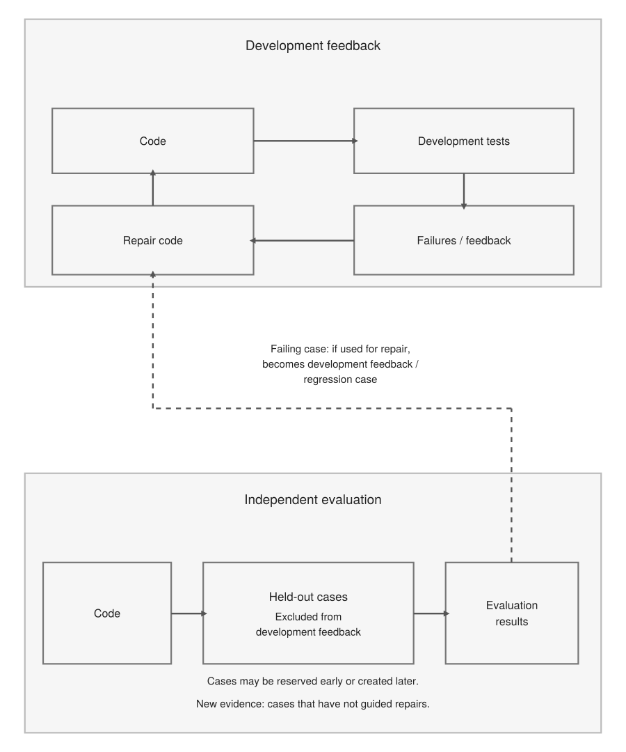
Without human involvement in the coding, more of the burden falls on test cases unseen during LLM code generation. When we cannot assume that the code does not special-case familiar inputs or have arbitrary failure modes, we need something closer to exhaustive testing to ensure code correctness. When exhaustive testing is not practical, we can use held-out evaluation tests, serving the purpose of test data in ML model evaluation. Here, held-out means excluded from the LLM’s development feedback loop, whether reserved early or created later (Kapoor & Narayanan, 2023). A failing case pasted back to the LLM for repair becomes development feedback, not an unseen evaluation test. It can join the regression suite, but independent evidence must come from cases that have not guided those repairs.
6 Expected Cost of Bugs
If we assume that every code out there has a non-zero risk of surfacing bugs in production, we can model when bugs appear using a time-to-event model. The events here are production bug incidents, not the latent defects in the code. One defect may cause several incidents, while another may never be triggered. Let \(v\in[0,1]\) denote the level of LLM use and \(q(v)\) the initial software quality at deployment, measured by the generic quality \(q\) introduced earlier. For simplicity, suppose that the deployment environment \(E\) remains fixed over a time horizon \(T\). We model incidents as a homogeneous Poisson process, so the count of all incidents satisfies
\[ N(T) \mid q(v),E \sim \operatorname{Poisson}\bigl(\lambda(q(v),E)\cdot T\bigr). \]
The rate \(\lambda(q(v),E)\) is the recurrent incident intensity: the expected number of incidents per unit time (e.g. a month) and the hazard of each inter-incident waiting time, including the wait to the first incident. We assume that the hazard \(\lambda\) is a monotonically decreasing function of \(q(v)\), so that lower-quality software has a higher risk of surfacing bugs.
But incident frequency is only one part of risk. Let the random cost of an incident be
\[ C=C_{\mathrm{fix}}+C_{\mathrm{business}}, \qquad \mu(q(v),E)=\mathbb{E}[C\mid q(v),E]. \]
The fixing cost \(C_{\mathrm{fix}}\) includes diagnosing, repairing, testing, and deploying the fix. The business cost \(C_{\mathrm{business}}\) includes consequences such as downtime, lost revenue, wrong decisions, and liability. A broken page on my personal website may have little business cost. A bug affecting a clinical dosing decision or a regulatory submission could cause patient harm, delays or legal consequences. The domain and criticality of the application, represented in \(E\), therefore matter even when two systems have the same incident rate.
Assume that, conditional on \(q(v)\) and \(E\), incident costs \(C_i\) are independent and identically distributed with finite means, and independent of the incident count. If costs are additive, the total cost over \(T\) is \(L(T)=\sum_{i=1}^{N(T)}C_i\), with zero cost when there are no incidents. Its expected value is
\[ \begin{aligned} \mathbb{E}[L(T)\mid q(v),E] &=\lambda(q(v),E)\cdot T\mu(q(v),E)\\ &=\lambda_0(E)\cdot e^{-\beta q(v)}\cdot T \left(\mathbb{E}[C_{\mathrm{fix}}\mid q(v),E] +\mathbb{E}[C_{\mathrm{business}}\mid q(v),E]\right). \end{aligned} \]
This separates how often incidents occur from how costly they are. Higher initial quality reduces the incident rate in this model, but its effect on expected total cost also depends on the cost per incident. The stationarity and independence assumptions simplify reality: updates can change quality, and incidents can cluster or have overlapping consequences. Finally, expected cost alone does not capture catastrophic tail risk. In a high-risk domain, a rare but devastating incident may be unacceptable even when the average cost looks small. However, the above model is sufficient to demonstrate the main point of this blog post.
7 Optimizing the Level of LLM Use
7.1 A Baseline Without Development Costs
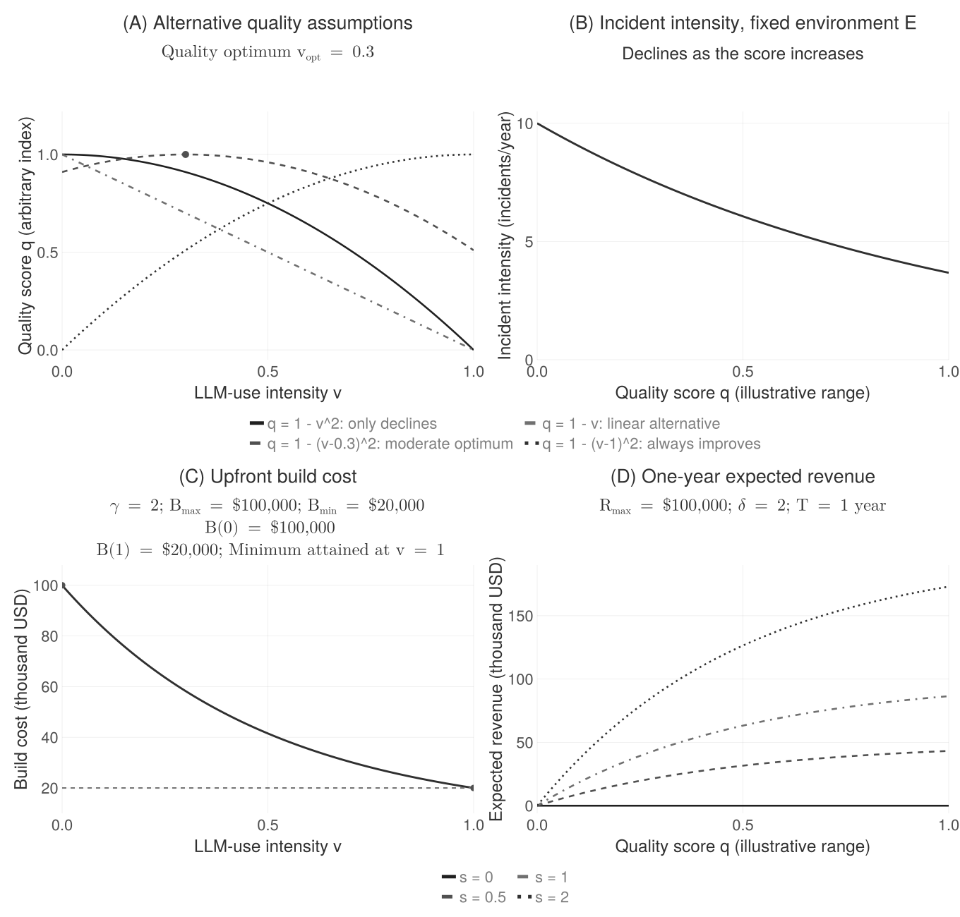
Suppose I start with the simplest version of the story: more LLM use lowers the initial code quality \(q(v)\), which raises the incident rate \(\lambda(q(v),E)\) and possibly the expected total cost \(\mathbb{E}[L(T)\mid q(v),E]\). That is an assumption for this scenario, not a claim that all LLM use harms quality; how much it does depends on oversight and review. As one concrete choice, let \(q(v)\) decrease quadratically with the level of LLM use \(v\):
\[ q(v) = q_{\max} - \alpha v^2, \] Here \(q_{\max}\) is the best initial quality available without LLM use, and \(\alpha>0\) sets how strongly LLM use affects quality. In this scenario, as \(v\) rises, \(q(v)\) falls, so the incident rate rises and expected total cost may rise with it.
With no other constraints in play, minimizing the expected total cost over \(v\) gives the optimal level of LLM use \(v^*\):
\[ v^* = \arg\min_v \mathbb{E}[L(T)\mid q(v),E]. \]
For simplicity, suppose the expected cost per incident \(\mu(q(v),E)\) does not depend on \(q(v)\), so that \[ \mathbb{E}[L(T)\mid q(v),E] = \lambda(q(v),E)\cdot T \mu(E). \] Then the optimization only has to minimize the incident rate in \(v\): \[ v^* = \arg\min_{v\in[0,1]} \lambda(q(v),E). \] Since \(\lambda(q(v),E)\) decreases in \(q(v)\) and \(q(v)\) decreases in \(v\), the incident rate increases in \(v\), so the optimum sits at \[ v^* = 0, \] In this simplified model manual coding wins, and the optimum is unique as long as \(T>0\) and \(\mu(E)>0\); if either is zero, every level of LLM use ties.
The assumptions behind that conclusion are:
- The software will be used for time \(T\).
- There is no additional cost to taking a long time to build the software manually.
- There is no additional cost to using the LLM.
- The cost of building the software is independent of LLM use.
- The revenue is independent of the level of LLM use.
- The initial code quality \(q(v)\) is a decreasing function of the level of LLM use \(v\).
- The expected cost per incident \(\mu(q(v),E)\) is constant with respect to \(q(v)\).
- The incident rate \(\lambda(q(v),E)\) is a decreasing function of \(q(v)\).
For software being developed from scratch, of course, several of these assumptions break down, so let me relax them one at a time. The most obvious is the cost of building the software itself, which I had set aside as small next to the cost of incidents.
7.2 Relaxing the Assumptions
Picture a startup building new software, with about one year to produce the best version it can in order to either:
- Sign up prospective users, or
- Secure investment.
Either way it needs a working proof of concept that shows the idea is viable. Suppose too that the startup is short on resources. In this scenario, I let the initial quality \(q(v)\) follow a concave quadratic in the level of LLM use \(v\), so that some LLM use helps quality up to a point and hurts it past that point: \[ q(v) = q_{\max} - \alpha\cdot(v - v_{\text{opt}})^2, \] Here \(q_{\max}\) is the best initial quality, \(v_{\text{opt}}\) is the level of LLM use that reaches it, and \(\alpha>0\) sets how quickly quality falls off as use moves away from \(v_{\text{opt}}\).
I take the build cost to fall as LLM use rises, quickly at first and then more slowly, rather than to rise. A normalized exponential pinned to a maximum at \(v=0\) and a minimum at \(v=1\) captures that: \[ B(v) = B_{\min} + (B_{\max}-B_{\min})\frac{e^{-\gamma v}-e^{-\gamma}}{1-e^{-\gamma}}, \] Here \(B_{\max}=B(0)\) is the no-LLM build cost, \(B_{\min}=B(1)\) with \(0<B_{\min}<B_{\max}\) is the cheapest build, and \(\gamma>0\) sets how fast the cost falls. The cost is strictly decreasing in \(v\): it drops fastest at small \(v\), flattens as \(v\to1\), and reaches \(B_{\min}\) exactly at \(v=1\). It helps to collect the constants as \[ \Lambda=\frac{B_{\max}-B_{\min}}{1-e^{-\gamma}}, \] so that \(B(v)=B_{\min}+\Lambda\cdot\left(e^{-\gamma v}-e^{-\gamma}\right)\) and \(B'(v)=-\Lambda\gamma\cdot e^{-\gamma v}<0\).
Revenue is uncertain too: a startup’s idea can fail even when the software works well. I model expected revenue as rising with initial quality but flattening out, since extra quality brings diminishing returns. The reference curve is \[ R(q(v)) = R_{\max}\cdot\left(1 - e^{-\delta q(v)}\right), \] where \(R_{\max}>0\) is the reference revenue ceiling and \(\delta>0\) sets how fast revenue grows with quality. To look at uncertainty or market size, I add a scalar multiplier \(s\geq0\): \[ R_s(q)=s\cdot R_{\max}\cdot\left(1-e^{-\delta q}\right). \] If failure earns nothing and the reference curve is conditional on success, then \(s=p\in[0,1]\) is a constant success probability that I assume is independent of both \(v\) and \(q\). More generally \(s>1\) stands for a larger market or upside scale, not a probability. If \(R_{\max}\) already bakes success probability into expected revenue, multiplying by it again would double-count. The derivations and numbers below use the \(s=1\) reference case, which is a normalization, not a claim that success is certain. One of the later sensitivity subsections varies \(s\) with everything else held fixed.
I keep the earlier simplifying assumption that the expected per-incident cost \(\mu(E)\) does not depend on \(q(v)\). Writing the incident hazard explicitly, \[ \lambda(q(v),E)=\lambda_0(E)\cdot e^{-\beta q(v)}, \qquad \beta>0. \] For fixed environment \(E\) and deployment horizon \(T\), define \[ A=T\lambda_0(E)\cdot \mu(E)>0, \qquad \mathbb{E}[L(T)\mid q(v),E]=A\cdot e^{-\beta q(v)}. \] Revenue and costs are all measured over the same deployment horizon \(T\), and the upfront build cost is charged to that horizon. The startup’s one-year development window is a different thing from this deployment horizon. When I vary \(s\), build and incident costs stay fixed: the spending and operation over the assumed horizon happen even if the idea flops commercially.
Expected net profit is just expected revenue minus expected total cost (at \(s=1\) here): \[ \Pi_{\mathrm{base}}(v) = R(q(v)) - B(v) - \mathbb{E}[L(T)\mid q(v),E] \] where \(\Pi_{\mathrm{base}}(v)\) is expected net profit as a function of LLM use \(v\). Plugging in \(R(q(v))\), \(B(v)\), and \(\mathbb{E}[L(T)\mid q(v),E]\) lets me see how the level of LLM use moves profitability.
Equivalently, I can minimize the net economic loss \[ J(v)=B(v)+\mathbb{E}[L(T)\mid q(v),E]-R(q(v))=-\Pi_{\mathrm{base}}(v). \] Unlike the random incident-only loss \(L(T)\), \(J(v)\) also includes the build cost and subtracts revenue, so it can go negative when the product is profitable.
7.3 The Profit-Maximizing Level
Substituting gives the optimization problem \[ \begin{aligned} \Pi_{\mathrm{base}}(v)&=R_{\max}\cdot\left(1-e^{-\delta q(v)}\right)-B_{\min}-\Lambda\cdot\left(e^{-\gamma v}-e^{-\gamma}\right)-A\cdot e^{-\beta q(v)},\\ v^*&=\arg\max_{v\in[0,1]}\Pi_{\mathrm{base}}(v). \end{aligned} \] Since \(q'(v)=-2\alpha\cdot(v-v_{\text{opt}})\), differentiating gives \[ \Pi_{\mathrm{base}}'(v)=\Lambda\gamma\cdot e^{-\gamma v} -2\alpha\cdot(v-v_{\text{opt}}) \left[\delta R_{\max}\cdot e^{-\delta q(v)}+\beta A\cdot e^{-\beta q(v)}\right]. \] To tidy this up, I write the marginal economic value of quality as \[ H(q)=\delta R_{\max}\cdot e^{-\delta q}+\beta A\cdot e^{-\beta q}>0. \] Then the derivative is \[ \Pi_{\mathrm{base}}'(v)=\Lambda\gamma\cdot e^{-\gamma v} -2\alpha\cdot(v-v_{\text{opt}})\cdot H(q(v)). \] For \(v\leq v_{\text{opt}}\) the derivative is strictly positive, since build costs fall while quality improves or stays flat. So the profit optimum sits strictly to the right of the quality optimum unless \(v_{\text{opt}}=1\), and in particular \(v=0\) cannot be optimal here when \(B_{\max}>B_{\min}\).
Differentiating once more to see the curvature and the monotonicity, \[ \begin{aligned} \Pi_{\mathrm{base}}''(v)={}&-\Lambda\gamma^2\cdot e^{-\gamma v}-2\alpha\cdot H(q(v))\\ &-4\alpha^2\cdot(v-v_{\text{opt}})^2 \left[\delta^2\cdot R_{\max}\cdot e^{-\delta q(v)}+\beta^2\cdot A\cdot e^{-\beta q(v)}\right]<0. \end{aligned} \]
7.4 Monotone Expected Profit: Necessary and Sufficient Conditions
So expected profit is strictly concave and \(\Pi_{\mathrm{base}}'\) strictly decreasing on \([0,1]\), which gives \(\Pi_{\mathrm{base}}'(1)\leq\Pi_{\mathrm{base}}'(v)\leq\Pi_{\mathrm{base}}'(0)\) for every \(v\in[0,1]\). Then \(\Pi_{\mathrm{base}}'(1)\geq0\) forces \(\Pi_{\mathrm{base}}'(v)\geq0\) everywhere; the same argument at \(v=0\) handles the nonpositive case. A continuously differentiable function is nondecreasing on an interval exactly when its derivative is nonnegative throughout, and nonincreasing exactly when the derivative is nonpositive throughout. Under the stated assumptions, then, these conditions are both necessary and sufficient:
- Expected profit is nondecreasing on \([0,1]\) if and only if \[ \bigl[\forall v\in[0,1],\ \Pi_{\mathrm{base}}'(v)\geq0\bigr] \quad\Longleftrightarrow\quad \Pi_{\mathrm{base}}'(1)\geq0 \quad\Longleftrightarrow\quad \Lambda\geq\frac{2\alpha\cdot(1-v_{\text{opt}})\cdot e^\gamma}{\gamma}H(q(1)). \] The unique optimum is \(v^*=1\) (full LLM use). Recall that \(\Lambda=(B_{\max}-B_{\min})/(1-e^{-\gamma})\) scales the build-cost saving. When \(v_{\text{opt}}=1\), the threshold is zero, so every allowed \(\Lambda>0\) satisfies it.
- Expected profit would be nonincreasing on \([0,1]\) if and only if \[ \bigl[\forall v\in[0,1],\ \Pi_{\mathrm{base}}'(v)\leq0\bigr] \quad\Longleftrightarrow\quad \Pi_{\mathrm{base}}'(0)\leq0 \quad\Longleftrightarrow\quad \Lambda\gamma+2\alpha v_{\text{opt}}\cdot H(q(0))\leq0. \] This condition is impossible under the stated assumptions, as shown below.
Here \(q(0)=q_{\max}-\alpha v_{\text{opt}}^2\) and \(q(1)=q_{\max}-\alpha\cdot(1-v_{\text{opt}})^2\) are the quality values at the two endpoints, \(v=0\) and \(v=1\). The endpoint test and the sign of \(\Pi_{\mathrm{base}}'\) on the whole interval are equivalent in both directions. Necessity is immediate: \([0,1]\) contains its endpoints, so if \(\Pi_{\mathrm{base}}'(v)\geq0\) for every \(v\), then in particular \(\Pi_{\mathrm{base}}'(1)\geq0\), and if \(\Pi_{\mathrm{base}}'(v)\leq0\) for every \(v\), then in particular \(\Pi_{\mathrm{base}}'(0)\leq0\). Sufficiency comes from strict concavity, which makes \(\Pi_{\mathrm{base}}'\) strictly decreasing, so \(\Pi_{\mathrm{base}}'(1)\geq0\) forces \(\Pi_{\mathrm{base}}'(v)\geq0\) for every \(v\leq1\), and \(\Pi_{\mathrm{base}}'(0)\leq0\) forces \(\Pi_{\mathrm{base}}'(v)\leq0\) for every \(v\geq0\). The endpoint inequality can hold with equality, meaning the derivative is exactly zero at \(v=1\) or at \(v=0\). Even then strict concavity (\(\Pi_{\mathrm{base}}''<0\)) makes \(\Pi_{\mathrm{base}}'\) strictly decreasing, so a zero at \(v=1\) still forces \(\Pi_{\mathrm{base}}'(v)>0\) for every \(v<1\), and a zero at \(v=0\) forces \(\Pi_{\mathrm{base}}'(v)<0\) for every \(v>0\). Profit is still strictly monotone, the endpoint stays the unique maximizer, and the curve never flattens into a tie or a plateau. Finally, since \(J=-\Pi_{\mathrm{base}}\) we have \(J'=-\Pi_{\mathrm{base}}'\), so the two functions move in opposite directions: the condition for nondecreasing profit is exactly the condition for nonincreasing loss, and vice versa, with the same strictness in the interior.
It turns out that nonincreasing expected profit is impossible under this quadratic startup model. Suppose \(\Pi_{\mathrm{base}}'(v)\leq0\) for every \(v\in[0,1]\). At \(v=0\) that would require \(\Pi_{\mathrm{base}}'(0)\leq0\), but \[ \Pi_{\mathrm{base}}'(0)=\Lambda\gamma+2\alpha v_{\text{opt}}\cdot H(q(0))\geq \Lambda\gamma>0, \] a contradiction, since \(v_{\text{opt}}\geq0\), \(\alpha>0\), and \(H>0\). When \(v_{\text{opt}}=0\), the same contradiction holds with \(\Pi_{\mathrm{base}}'(0)=\Lambda\gamma>0\). Continuity of \(\Pi_{\mathrm{base}}'\) then also gives some \(\varepsilon\in(0,1]\) with \(\Pi_{\mathrm{base}}'(v)>0\) throughout \([0,\varepsilon)\), so this is not just an endpoint fact. Early on, build-cost savings and nondecreasing quality both push toward more LLM use. Expected profit either rises across the whole interval or has a single interior peak.
Hypothetically, a capable enough LLM might keep improving quality all the way to full use. In the quadratic model, that is the special case \(v_{\text{opt}}=1\): quality rises for \(v<1\) and has zero slope at \(v=1\). More generally, if \(q'(v)\geq0\) throughout \([0,1]\), the assumptions I already made (falling build costs, quality-linked revenue, declining incident rates, and a fixed expected cost per incident) give \[ \Pi_{\mathrm{base}}'(v)=H(q(v))\cdot q'(v)+\Lambda\gamma\cdot e^{-\gamma v}>0, \qquad v^*=1. \] Then every extra bit of LLM use helps the modeled financial outcome. That would be a qualitative regime change, a kind of break-even capability threshold for the quality trade-off. It is a theoretical possibility, not a property I claim for current LLMs.
And this holds only for the original model without debt penalties or constraints; once debt costs enter, they can matter even at \(v_{\text{opt}}=1\) and overturn full use.
7.5 Nonmonotone Expected Profit: An Interior Optimum
An interior optimum appears exactly when \(\Pi_{\mathrm{base}}'(0)>0>\Pi_{\mathrm{base}}'(1)\). Since \(\Pi_{\mathrm{base}}'\) is continuous and strictly decreasing, there is then one root \(\Pi_{\mathrm{base}}'(v^*)=0\): profit rises and then falls, while loss falls and then rises. For the quadratic quality model \(\Pi_{\mathrm{base}}'(0)>0\) always holds, so the condition on the parameters is \[ \Lambda\gamma\cdot e^{-\gamma}<2\alpha\cdot(1-v_{\text{opt}})\cdot H(q(1)). \] The root lies in \((v_{\text{opt}},1)\) and satisfies the stationarity condition \(\Pi_{\mathrm{base}}'(v^*)=0\), the point where the derivative in \(v\) is zero: \[ \Lambda\gamma\cdot e^{-\gamma v^*} =2\alpha\cdot(v^*-v_{\text{opt}}) \left[\delta R_{\max}\cdot e^{-\delta q(v^*)}+\beta A\cdot e^{-\beta q(v^*)}\right]. \] The left side is the marginal saving in build cost, and the right side is the marginal revenue lost through lower quality plus the extra expected incident cost. This balance has no general elementary closed form, so after checking the boundary condition, I solve \(\Pi_{\mathrm{base}}'(v)=0\) numerically by bisection on \([v_{\text{opt}},1]\), where the derivative is continuous, strictly decreasing, and changes sign.
With everything else held fixed, higher expected incident costs or a longer deployment horizon raise \(A=T\cdot \lambda_0(E)\cdot \mu(E)\), the horizon-total scale of expected incident loss, and pull the optimum toward the quality-maximizing level \(v_{\text{opt}}\). A larger \(R_{\max}\) does the same. A larger maximum cost \(B_{\max}\) (equivalently a larger \(\Lambda=(B_{\max}-B_{\min})/(1-e^{-\gamma})\)) pushes the other way, toward more LLM use. The optimum can stay pinned at a boundary until this balance shifts; once it is interior, a shift moves it. For the horizon comparison, I hold the horizon-total revenue parameters fixed. So the quality-maximizing \(v_{\text{opt}}\) and the profit-maximizing \(v^*\) are different decisions: giving up some quality can pay off when it buys enough development savings.
In this illustrative model, LLM use lowers development costs, and moderate use can also improve quality. Past the best-quality level, further build savings have to be weighed against lost revenue and costlier bugs later. The most profitable choice can therefore use more LLM help than the choice that gives the highest quality.
7.6 When LLM Use Can Only Hurt Quality Under the Model
Setting \(v_{\text{opt}}=0\) in the original quadratic model gives \[ q(v)=q_{\max}-\alpha v^2,\qquad q'(v)=-2\alpha v. \] Then any positive amount of LLM use lowers quality relative to manual coding, and quality falls strictly for \(v>0\), though its derivative at zero is still zero. I mean this as an illustrative assumption about unreviewed generated work, not as a claim that all LLM use harms quality.
The expected profit derivative becomes \[ \Pi_{\mathrm{base}}'(v)=\Lambda\gamma\cdot e^{-\gamma v}-2\alpha v\cdot H(q_{\max}-\alpha v^2), \qquad \Pi_{\mathrm{base}}'(0)=\Lambda\gamma>0. \] So zero is not the economic optimum when \(B_{\max}>B_{\min}\), even though LLM use only hurts quality here: near zero, the quality penalty is quadratic while the build saving is first-order. Strict concavity still holds, so profit rises and \(v^*=1\) exactly when \[ 2\alpha\cdot H(q_{\max}-\alpha)\leq \Lambda\gamma\cdot e^{-\gamma}; \] otherwise there is a single interior root in \((0,1)\). Outside the strict \(B_{\max}>B_{\min}\) case, if \(B_{\max}=B_{\min}\) there is no build saving at all, and then \(\Pi_{\mathrm{base}}'(v)=-2\alpha v\cdot H(q(v))<0\) for \(v>0\) with \(v^*=0\), as long as quality has positive economic value (\(H>0\), as it does for the revenue and incident parameters assumed here).
7.7 Allowing a Manual Optimum: A Different Quality Assumption
To allow the other extreme, I replace the quadratic quality curve with a separate, monotonically decreasing linear one: \[ q(v)=q_{\max}-\alpha v,\qquad \alpha>0. \] The build-cost, revenue, and incident assumptions stay the same. Unlike the quadratic case with \(v_{\text{opt}}=0\), this curve has a nonzero initial quality penalty \(q'(0)=-\alpha\), so \[ \begin{aligned} \Pi_{\mathrm{base}}'(v)&=\Lambda\gamma\cdot e^{-\gamma v}-\alpha\cdot H(q(v)),\\ \Pi_{\mathrm{base}}''(v)&=-\Lambda\gamma^2\cdot e^{-\gamma v} -\alpha^2\left[\delta^2\cdot R_{\max}\cdot e^{-\delta q(v)}+\beta^2\cdot A\cdot e^{-\beta q(v)}\right]<0. \end{aligned} \] Here again \(\Pi_{\mathrm{base}}'\) is strictly decreasing, so \(\Pi_{\mathrm{base}}'(1)\leq\Pi_{\mathrm{base}}'(v)\leq\Pi_{\mathrm{base}}'(0)\) for every \(v\in[0,1]\). Substituting the endpoint derivatives gives these necessary and sufficient conditions for the linear variant:
- Expected profit is nondecreasing on \([0,1]\) if and only if \[ \bigl[\forall v\in[0,1],\ \Pi_{\mathrm{base}}'(v)\geq0\bigr] \quad\Longleftrightarrow\quad \Lambda\gamma\cdot e^{-\gamma}\geq\alpha\cdot H(q_{\max}-\alpha), \] giving the unique full LLM use optimum \(v^*=1\).
- Expected profit is nonincreasing on \([0,1]\) if and only if \[ \bigl[\forall v\in[0,1],\ \Pi_{\mathrm{base}}'(v)\leq0\bigr] \quad\Longleftrightarrow\quad \Lambda\gamma\leq\alpha\cdot H(q_{\max}), \] giving the unique no LLM use optimum \(v^*=0\).
- Expected profit has a unique interior peak if and only if \[ \alpha\cdot H(q_{\max})<\Lambda\gamma \quad\text{and}\quad \Lambda\gamma\cdot e^{-\gamma}<\alpha\cdot H(q_{\max}-\alpha). \] The intermediate LLM use optimum is the unique root of \(\Lambda\gamma\cdot e^{-\gamma v^*}=\alpha\cdot H(q_{\max}-\alpha v^*)\) in \((0,1)\).
This change to the quality curve makes a no-LLM-use optimum possible. For the numerical illustration below, the linear variant uses the same normalized build-cost form with \(B_{\max}=\$30{,}000\), \(B_{\min}=\$20{,}000\), and \(\gamma=2\).
7.8 Numerical Examples
For an illustrative revenue-generating startup, take the values below. Money is in USD, and \(T=1\) deployment year, separate from the development window.
| Parameters | Assumed values |
|---|---|
| Quality | \(q_{\max}=1\), \(\alpha=1\), \(v_{\text{opt}}=0.3\) |
| Build cost | \(B_{\max}=\$100{,}000\), \(B_{\min}=\$20{,}000\), \(\gamma=2\) |
| Revenue | \(R_{\max}=\$100{,}000\), \(\delta=2\) |
| Incidents | \(\lambda_0(E)=10\) incidents/year, \(\beta=1\) |
| Mean incident cost | \(\mu(E)=\$5{,}000\) (\(\$1{,}000\) fixing + \(\$4{,}000\) business cost) |
Quality here is a dimensionless index, not a percentage of correct code or an uptime guarantee: \(q(v)=1-(v-0.3)^2\) ranges from \(0.51\) to \(1\). The build budget, revenue ceiling, and incident costs describe a modest commercial product with repairable disruptions, not catastrophic ones. The incident-rate scale is \(\lambda_0(E)=10\) incidents/year, so at peak quality \(q_{\max}=1\) (with \(\beta=1\)) the incident rate is \(\lambda_0(E)\cdot e^{-\beta q_{\max}}=10e^{-1}\approx3.68\) incidents/year, and \(A=T\cdot \lambda_0(E)\cdot \mu(E)=\$50{,}000\).
Substituting into the first-order condition gives, with monetary coefficients in USD, \[ 185{,}042.82e^{-2v} =2(v-0.3)\left[200{,}000e^{-2[1-(v-0.3)^2]}+50{,}000e^{-[1-(v-0.3)^2]}\right]. \] Here \(J'(0)\approx-216{,}562\) and \(J'(1)\approx117{,}958\) USD per unit of \(v\), so the loss is nonmonotone. Solving numerically gives \(v^*\approx0.6945934\), about 69% on the model’s LLM-use intensity scale. This is the unique minimizer of \(J\), and so the maximizer of \(\Pi_{\mathrm{base}}\). At that optimum:
- Quality: \(q(v^*)\approx0.844\).
- Expected annual incident count: \(\lambda(q(v^*),E)\cdot T\approx4.299\).
- Expected revenue: \(\$81{,}522\); upfront build cost: \(\$30{,}542\); expected incident loss: \(\$21{,}493\).
- Net profit: \(\Pi_{\mathrm{base}}(v^*)\approx\$29{,}487\).
- Net economic loss: \(J(v^*)\approx-\$29{,}487\).
| Choice | \(v\) | Net profit over the deployment year |
|---|---|---|
| No LLM use | 0.000 | \(-\$36{,}329\) |
| Maximum quality | 0.300 | \(\$9{,}817\) |
| Maximum profit | 0.695 | \(\$29{,}487\) |
| Full LLM use | 1.000 | \(\$13{,}916\) |
Moving past the quality optimum saves enough build cost to raise profit, but going all the way to \(v=1\) gives up too much revenue and adds incident losses. At this lower revenue ceiling, abandoning LLM use is itself a loss: the no-use choice is negative, and full use earns less than the interior optimum. The best balance is interior for these assumptions, though that is not a general recommendation.
For the quality-only-worsens quadratic case, I change only \(v_{\text{opt}}\) to \(0\) and keep every other baseline parameter, including \(B_{\max}=\$100{,}000\), \(B_{\min}=\$20{,}000\), and \(A=\$50{,}000\). Then \(q(v)=1-v^2\), \(J'(0)=-185{,}043\), and \(J'(1)\approx474{,}957\) USD per unit of \(v\). The unique root is \(v^*\approx0.4995565\), with quality \(q\approx0.750443\), expected annual incident count \(\approx4.722\), and net profit \(\Pi_{\mathrm{base}}(v^*)\approx\$12{,}553\), compared with \(-\$31{,}928\) at \(v=0\). Even under this hypothetical quality penalty for unreviewed coding, build savings make some LLM use profitable, and no LLM use would lose money at this revenue ceiling.
For an optimum at full LLM use with the original quadratic quality curve, go back to the baseline \(v_{\text{opt}}=0.3\) and hold every baseline parameter fixed except the maximum build cost \(B_{\max}\). Written in terms of that maximum cost, the endpoint condition requires \[ B_{\max}\geq B_{\min}+\frac{2\alpha\cdot(1-v_{\text{opt}})\cdot H(q(1))\cdot e^\gamma\cdot(1-e^{-\gamma})}{\gamma} \approx\$476{,}821.58. \] Take \(B_{\max}=\$1{,}000{,}000\) (with \(B_{\min}=\$20{,}000\)): then \(J'(1)\approx-163{,}773<0\), so loss falls throughout \([0,1]\) and \(v^*=1\), with full LLM use profitable at \(\Pi_{\mathrm{base}}(1)\approx\$13{,}916\).
For an optimum at no LLM use, which needs the modified linear quality assumption, I use \(q(v)=1-v\) and the same other parameters, with the linear-variant build costs \(B_{\max}=\$30{,}000\) and \(B_{\min}=\$20{,}000\). Then \(\alpha\cdot H(q_{\max})\approx\$45{,}461>\Lambda\gamma=\$23{,}130\), so \(J'(0)\approx22{,}331>0\). Loss rises throughout the interval and \(v^*=0\).
These hypothetical regimes sum up the trade-off; the derivative values are in USD per unit of \(v\):
| Quality model | Build cost | \(J'(0)\) | \(J'(1)\) | Loss shape and unique optimum |
|---|---|---|---|---|
| Original quadratic, \(v_{\text{opt}}=0.3\) | \(B_{\max}=\$100{,}000\) | \(-216{,}562\) | \(117{,}958\) | Falls then rises; \(v^*\approx0.6945934\) |
| Original quadratic, \(v_{\text{opt}}=0\) | \(B_{\max}=\$100{,}000\) | \(-185{,}043\) | \(474{,}957\) | Falls then rises; \(v^*\approx0.4995565\) |
| Original quadratic, \(v_{\text{opt}}=0.3\) | \(B_{\max}=\$1{,}000{,}000\) | \(-2{,}298{,}293\) | \(-163{,}773\) | Decreases; \(v^*=1\) |
| Modified linear | \(B_{\max}=\$30{,}000\) | \(22{,}331\) | \(246{,}870\) | Increases; \(v^*=0\) |
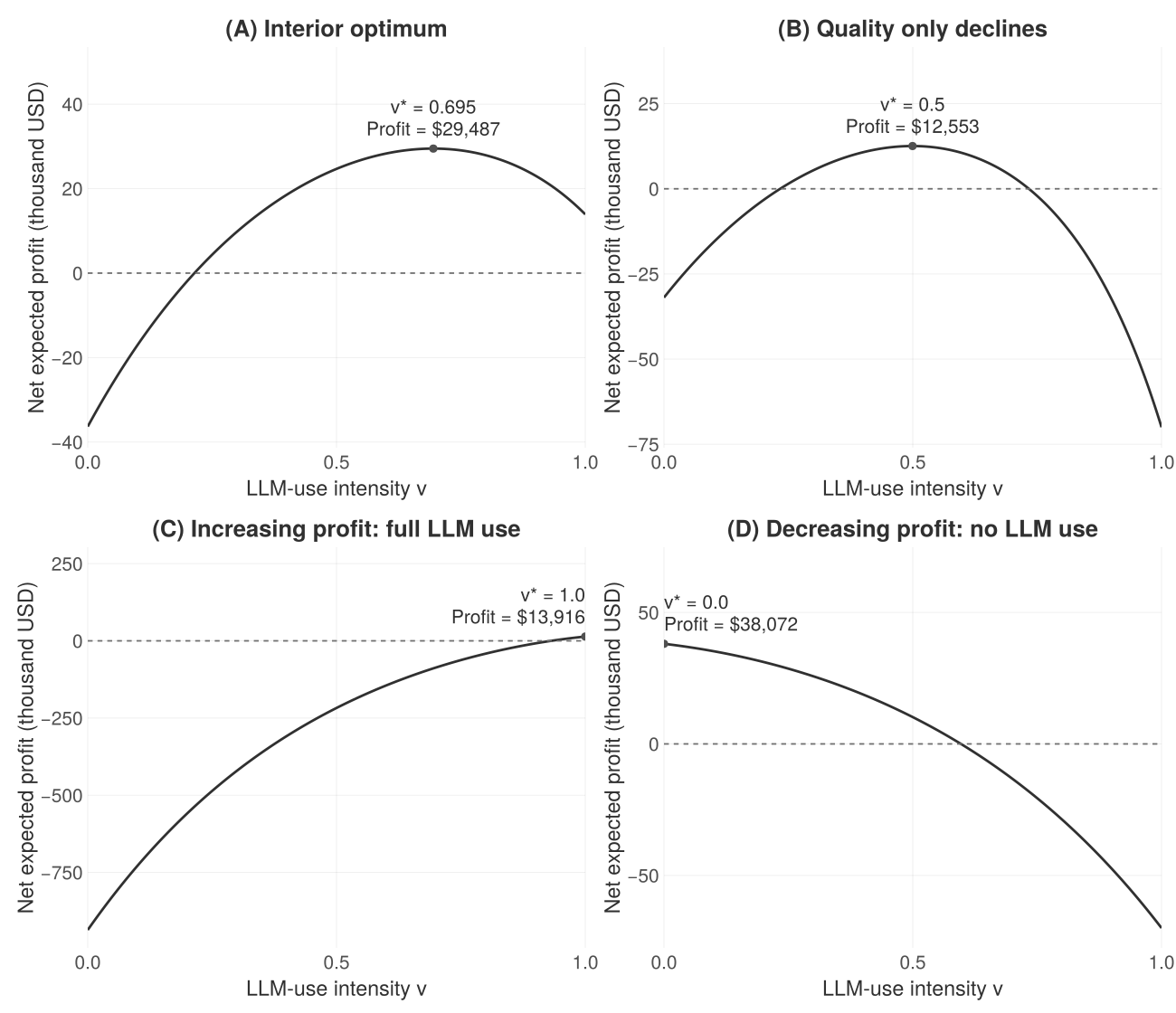
In the full LLM use case \(J(1)\approx-\$13{,}916\), a net profit, and in the modified linear no-LLM-use case \(J(0)\approx-\$38{,}072\). An optimal choice does not have to be profitable.
7.9 Sensitivity to Expected Revenue
For the original quadratic quality model, replacing reference revenue with \(R_s\) gives \[ \Pi_s(v)=s\cdot R_{\max}\cdot\left(1-e^{-\delta q(v)}\right)-B_{\min}-\Lambda\cdot\left(e^{-\gamma v}-e^{-\gamma}\right)-A\cdot e^{-\beta q(v)}, \] with derivative \[ \Pi_s'(v)=\Lambda\gamma\cdot e^{-\gamma v} -2\alpha\cdot(v-v_{\text{opt}}) \left[s\delta R_{\max}\cdot e^{-\delta q(v)}+\beta A\cdot e^{-\beta q(v)}\right]. \] The strict-concavity argument from before still holds for every \(s\geq0\): replacing \(R_{\max}\) by \(s\cdot R_{\max}\) in \(\Pi_{\mathrm{base}}''\) keeps \(\Pi_s''<0\). For an interior optimum \(v^*(s)>v_{\text{opt}}\) under \(B_{\max}>B_{\min}\), differentiating \(\Pi_s'(v^*(s))=0\) implicitly gives \[ \frac{dv^*}{ds} =\frac{2\alpha\cdot(v^*-v_{\text{opt}})\cdot \delta R_{\max}\cdot e^{-\delta q(v^*)}} {\Pi_s''(v^*)}<0. \] The numerator is positive and the denominator is negative, so more expected revenue pulls the optimum toward the quality-maximizing level \(v_{\text{opt}}\), while less expected revenue favors more LLM use. The unique optimum is nonincreasing in \(s\) across the whole range, so it always lies between \(v_{\text{opt}}\) and \(1\): full use for small \(s\), decreasing toward \(v_{\text{opt}}\) as \(s\) grows. As \(s\to\infty\), it tends to \(v_{\text{opt}}\). At \(s=0\), incident costs still punish quality loss, so the optimum can stay interior rather than go to full use.
For \(v_{\text{opt}}<1\), write \(q_1=q(1)\). Full LLM use is optimal if and only if \[ \Lambda\gamma\cdot e^{-\gamma}\geq2\alpha\cdot(1-v_{\text{opt}}) \left[s\delta R_{\max}\cdot e^{-\delta q_1}+\beta A\cdot e^{-\beta q_1}\right]. \] Equivalently, define \[ s_c=\frac{\dfrac{\Lambda\gamma\cdot e^{-\gamma}}{2\alpha\cdot(1-v_{\text{opt}})} -\beta A\cdot e^{-\beta q_1}} {\delta R_{\max}\cdot e^{-\delta q_1}}. \] If \(s_c\geq0\), the full-use optimum holds exactly for \(0\leq s\leq s_c\), and if \(s_c<0\) it never holds for \(s\geq0\). When \(v_{\text{opt}}=1\), quality and build savings both favor full LLM use, so \(v^*=1\) for every \(s\).
Using the same common parameters as the quadratic example (\(q_{\max}=\alpha=1\), \(v_{\text{opt}}=0.3\), \(B_{\min}=\$20{,}000\), \(\gamma=2\), \(R_{\max}=\$100{,}000\), \(\delta=2\), \(\beta=1\), and \(A=\$50{,}000\)), I vary only \(s\) and the maximum build cost \(B_{\max}\). The resulting optimal LLM-use intensities are:
| Revenue multiplier \(s\) | Baseline \(B_{\max}=\$100{,}000\) | Intermediate \(B_{\max}=\$220{,}000\) | High build cost \(B_{\max}=\$1{,}000{,}000\) |
|---|---|---|---|
| 0 | 0.8931 | 1.0000 | 1.0000 |
| 0.25 | 0.8135 | 0.9865 | 1.0000 |
| 0.5 | 0.7625 | 0.9296 | 1.0000 |
| 1 | 0.6946 | 0.8555 | 1.0000 |
| 2 | 0.6141 | 0.7673 | 1.0000 |
| 3 | 0.5645 | 0.7112 | 0.9806 |
At zero revenue the baseline optimum is still interior (\(v^*\approx0.8931\)), because bugs cost money even when the idea earns nothing and build savings do not outweigh incident costs all the way to full use. The intermediate and high-build scenarios stay at full use until \(s_c\approx0.203754\) and \(s_c\approx2.622055\), which come from substituting into the threshold above. More revenue makes quality worth more, so the interior choices move toward \(0.3\), not toward zero LLM use. These are illustrative model outputs, not empirical causal estimates or recommendations.
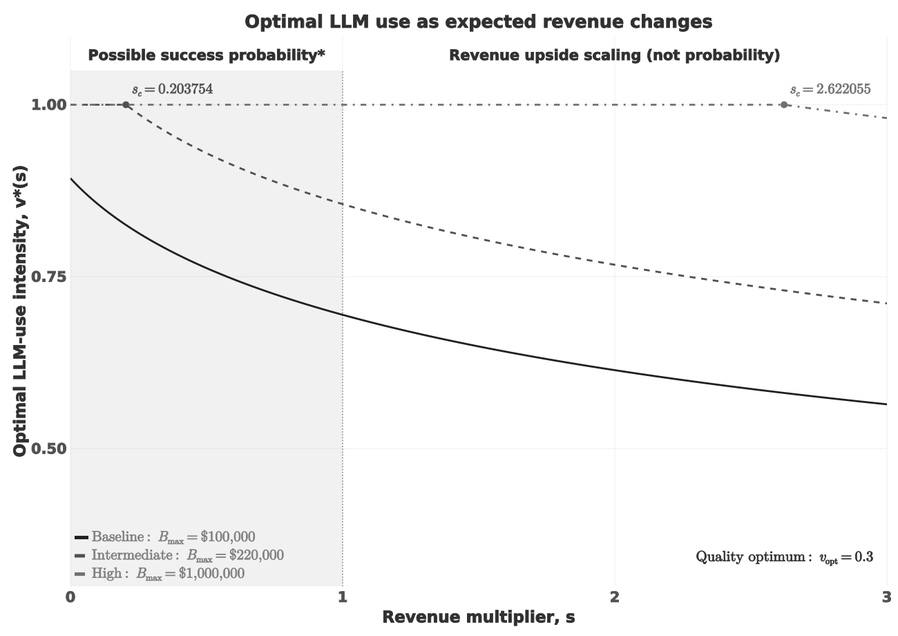
For the distinct linear quality variant, raising \(s\) also lowers the interior optimal level of LLM use, with boundary plateaus possible. Unlike the quadratic model, it can reach no LLM use, with threshold \(\Lambda\gamma\leq\alpha[s\delta R_{\max}\cdot e^{-\delta q_{\max}}+\beta A\cdot e^{-\beta q_{\max}}]\).
When better software can earn more, quality is worth more in this model. A low or uncertain payoff instead favors cheaper experimentation with more LLM use, with build and incident costs held fixed. That is a financial trade-off, not permission to relax safety standards: bugs can still cause harm even when a product earns nothing.
7.10 An Active Upfront Cost Constraint
A startup short on cash may face an upfront build-cost budget \(K\). For simplicity, this is a fixed cap on upfront spending, not on expected lifecycle cost. It is not a chance constraint either: that would bound the probability of a bad event, such as requiring the chance that spending exceeds a limit to be below some threshold, instead of fixing the amount available at build time. Expected bug costs stay in the profit objective but are not charged against the upfront budget. Going back to the original quadratic quality model, the problem becomes \[ v^*(K)=\arg\max_{v\in[0,1]}\Pi_s(v) \quad\text{subject to}\quad B(v)=B_{\min}+\Lambda\cdot\left(e^{-\gamma v}-e^{-\gamma}\right)\leq K. \] Because build cost strictly decreases with \(v\), the smallest attainable build cost is \(B(1)=B_{\min}\). Hence:
- If \(K<B_{\min}\), the problem is infeasible.
- If \(K\geq B_{\max}\), every \(v\in[0,1]\) is feasible; set \(v_{\min}(K)=0\).
- Otherwise, \(B_{\min}\leq K<B_{\max}\), so \(K-B_{\min}\geq0\). Recall that \(\Lambda=(B_{\max}-B_{\min})/(1-e^{-\gamma})\) sets the scale of the build-cost curve, since \(B(0)-B(1)=\Lambda\cdot(1-e^{-\gamma})=B_{\max}-B_{\min}\). The budget constraint becomes \[ B_{\min}+\Lambda\cdot\left(e^{-\gamma v}-e^{-\gamma}\right)\leq K \quad\Longleftrightarrow\quad e^{-\gamma v}\leq \frac{K-B_{\min}}{\Lambda}+e^{-\gamma}. \] The right-hand side is positive, because \(K\geq B_{\min}\) and \(e^{-\gamma}>0\). Taking logarithms, which are increasing, and dividing by \(-\gamma<0\) reverses the inequality, giving \[ v\geq v_K=-\frac{1}{\gamma}\ln\!\left(\frac{K-B_{\min}}{\Lambda}+e^{-\gamma}\right). \] With the definition of \(\Lambda\), the argument of the logarithm runs from \(e^{-\gamma}\) at \(K=B_{\min}\) to \(1\) at \(K=B_{\max}\), so \(v_K\in(0,1]\): it equals \(1\) at \(K=B_{\min}\) and falls to \(0\) as \(K\to B_{\max}\). The feasible interval is \([v_K,1]\); set \(v_{\min}(K)=v_K\).
Let \(v_u=\arg\max_{v\in[0,1]}\Pi_s(v)\) denote the unique optimum without the budget constraint. Strict concavity gives, whenever the budget is feasible, \[ v^*(K)=\max\{v_{\min}(K),v_u\}. \] The budget strictly distorts the choice exactly when \(K<B(v_u)\): it forces more LLM use than the unconstrained profit optimum and lowers the best achievable expected profit. If \(K=B(v_u)\), the constraint binds in the equality sense but does not change the choice, and its multiplier can be zero. For \(K>B(v_u)\), it is slack. So a binding constraint alone does not imply a strictly positive shadow price. The shadow price is the marginal value of relaxing the constraint: the extra optimal expected profit from one more unit of budget.
For a budget-bound optimum strictly inside the LLM-use interval, \(v^*=v_K\in(0,1)\), the Karush–Kuhn–Tucker conditions (Boyd & Vandenberghe, 2004; Kuhn & Tucker, 1951) use \[ \begin{aligned} \mathcal{L}(v,\eta)&=\Pi_s(v)+\eta\cdot\bigl(K-B(v)\bigr),\qquad \eta\geq0,\\ \Pi_s'(v^*)-\eta B'(v^*)&=0,\qquad \eta\cdot\bigl(K-B(v^*)\bigr)=0. \end{aligned} \] The scalar \(\eta\) is the Lagrange multiplier on the budget constraint, the dual variable associated with the upfront budget \(K\). Since \(B'(v)=-\Lambda\gamma\cdot e^{-\gamma v}\), \[ \eta=\frac{\Pi_s'(v^*)}{B'(v^*)} =-\frac{\Pi_s'(v^*)}{\Lambda\gamma\cdot e^{-\gamma v^*}}>0 \quad\text{when }v_K>v_u. \] At \(K=B_{\min}\) only \(v=1\) is feasible: the budget touches the upper bound \(v\leq1\), so the strict-feasibility constraint qualification fails. The multiplier formula derived above, \(\eta=-\Pi_s'(v^*)/(\Lambda\gamma\cdot e^{-\gamma v^*})\), assumes an interior budget-bound optimum \(v_K\in(0,1)\), so I do not apply it at this endpoint.
Writing \(V(K)=\Pi_s(v^*(K))\), the envelope theorem gives \(dV/dK=\eta\geq0\) under the usual conditions, with all other parameters fixed. This identifies the Lagrange multiplier \(\eta\) with the shadow price of the budget: it is the extra optimal expected profit from one more dollar of upfront budget, so relaxing a binding budget raises profit at rate \(\eta\), and tightening it lowers profit at that rate. Once the budget strictly distorts the choice, shrinking it forces more LLM use and lowers profit; that is a financing trade-off, not a claim that high LLM use maximizes quality.
For a worked example I keep all baseline parameters fixed at \(s=1\), \(q_{\max}=\alpha=1\), \(v_{\text{opt}}=0.3\), \(B_{\max}=\$100{,}000\), \(B_{\min}=\$20{,}000\), \(\gamma=2\), \(R_{\max}=\$100{,}000\), \(\delta=2\), \(\beta=1\), and \(A=\$50{,}000\) (so \(\Lambda=\$92{,}521.41\)). The unconstrained optimum \(v_u\approx0.6945934\) needs \(\$30{,}542.14\) upfront. A binding budget of \(K=\$28{,}000\) instead gives \[ \begin{aligned} v^*&=v_K=-\tfrac12\ln\!\left(\frac{28{,}000-20{,}000}{92{,}521.41}+e^{-2}\right)\approx0.7529856,\\ B(v^*)&=20{,}000+92{,}521.41\left(e^{-2v^*}-e^{-2}\right)=28{,}000,\\ q(v^*)&=1-(v^*-0.3)^2\approx0.794804,\\ \Pi_1(v^*)&=100{,}000(1-e^{-2q(v^*)})-28{,}000-50{,}000e^{-q(v^*)} \approx29{,}015.96. \end{aligned} \]
| Choice | LLM-use intensity \(v\) | Quality \(q(v)\) | Upfront build cost | Expected incident loss | Expected profit |
|---|---|---|---|---|---|
| Unconstrained optimum | 0.694593 | 0.844296 | \(\$30{,}542.14\) | \(\$21{,}492.99\) | \(\$29{,}486.92\) |
| Optimum with \(K=\$28{,}000\) | 0.752986 | 0.794804 | \(\$28{,}000.00\) | \(\$22{,}583.49\) | \(\$29{,}015.96\) |
The budget saves \(\$2{,}542.14\) upfront compared with the unconstrained choice, but expected profit falls by \(\$470.96\). Here \(\eta=-\Pi_1'(v_K)/(\Lambda\gamma\cdot e^{-\gamma v_K})\approx0.399139\), so one extra dollar of budget raises optimal expected profit by about \(\$0.40\) locally. The minimum feasible budget is \(B_{\min}=\$20{,}000\), and a \(\$19{,}000\) budget cannot fund any choice in this model. (A budget of \(K=\$31{,}000\) would be slack instead, since it exceeds the unconstrained upfront cost of \(\$30{,}542.14\), giving \(v^*\approx0.6945934\) and \(\eta=0\).)
A tight upfront budget can force more LLM use even when a lower-use approach would give higher quality and more expected profit. In practice, that can mean not being able to afford the human review that quality would call for. The budget limits what can be built now; it does not make the later cost of bugs go away.
7.11 Sensitivity to Incident Cost
What changes for a low-impact application where incidents are cheap? Write \(m=\mu(E)\geq0\) for the expected fixing plus business cost per incident, \(\mathcal{D}=T\cdot \lambda_0(E)>0\), and \(A(m)=\mathcal{D}m\). I hold all other environment and model parameters fixed, including the revenue multiplier \(s\geq0\), which isolates incident severity rather than frequency. The positive constants \(B_{\max},B_{\min},\gamma,\alpha,\beta,\delta,R_{\max}\) and the original quadratic quality curve \(q(v)=q_{\max}-\alpha\cdot(v-v_{\text{opt}})^2\) stay as they are, with \(v_{\text{opt}}\in[0,1]\). The net profit and its derivative can be written as \[ \begin{aligned} \Pi_m(v)&=s\cdot R_{\max}\cdot(1-e^{-\delta q(v)})-B_{\min}-\Lambda\cdot\left(e^{-\gamma v}-e^{-\gamma}\right) -\mathcal{D}m\cdot e^{-\beta q(v)},\\ \Pi_m'(v)&=\Lambda\gamma\cdot e^{-\gamma v}-2\alpha\cdot(v-v_{\text{opt}}) \left[s\delta R_{\max}\cdot e^{-\delta q(v)}+\beta \mathcal{D}m\cdot e^{-\beta q(v)}\right]. \end{aligned} \] Strict concavity survives even at \(m=0\) because \(B_{\max}>B_{\min}\), so write \(v^*(m)\) for the unique unconstrained maximizer on \([0,1]\). For an interior optimum with \(v_{\text{opt}}<1\), differentiating implicitly gives \[ \frac{dv^*}{dm} =\frac{2\alpha\cdot(v^*-v_{\text{opt}})\cdot \beta\mathcal{D}\cdot e^{-\beta q(v^*)}} {\Pi_m''(v^*)}<0. \] So cheaper incidents favor more LLM use, and the optimum is nonincreasing in \(m\) across the range, with possible full-use plateaus. But when \(s>0\) revenue still values quality, so even negligible incident cost does not have to make full use optimal.
Without an upfront budget limit, making each incident costlier pushes toward the LLM-use level that gives the best quality, with the other assumptions held fixed. That need not mean abandoning LLMs: under the illustrative assumptions the best-quality approach can still use some LLM help.
For \(v_{\text{opt}}<1\) and \(q_1=q(1)\), the endpoint condition gives the full-use threshold \[ m_c=\frac{\dfrac{\Lambda\gamma\cdot e^{-\gamma}}{2\alpha\cdot(1-v_{\text{opt}})} -s\delta R_{\max}\cdot e^{-\delta q_1}} {\beta\mathcal{D}\cdot e^{-\beta q_1}}. \] If the numerator is negative, full use is never optimal. Otherwise, it is optimal exactly for \(0\leq m\leq m_c\), equality included. As before, \(v_{\text{opt}}=1\) gives full use for every \(m\) instead.
7.12 The Limit of Vanishing Mean Incident Cost
The incident-loss term is \(\mathcal{D}m\cdot e^{-\beta q(v)}\). As \(m\downarrow0\) it shrinks uniformly to zero on the compact interval \([0,1]\), so \(\Pi_m\) converges uniformly to \(\Pi_{m=0}\) and the unique maximizer converges, \[ v^*(m)\longrightarrow v^*(0)\qquad(m\downarrow0). \]
At zero mean incident cost the marginal balance is \[ \Pi_{m=0}'(v)=\Lambda\gamma\cdot e^{-\gamma v} -2\alpha\cdot(v-v_{\text{opt}})\cdot s\delta R_{\max}\cdot e^{-\delta q(v)}. \] Full use is optimal exactly when \[ \Lambda\gamma\cdot e^{-\gamma}\geq 2\alpha\cdot(1-v_{\text{opt}})\cdot s\delta R_{\max}\cdot e^{-\delta q_1}, \] which for \(v_{\text{opt}}<1\) is equivalent to \(s\leq s_0=\frac{\Lambda\gamma\cdot e^{-\gamma+\delta q_1}}{2\alpha\cdot(1-v_{\text{opt}})\cdot \delta R_{\max}}\); otherwise \(v^*(0)\) is the unique root of \(\Pi_{m=0}'(v)=0\) in \((v_{\text{opt}},1)\). If \(s=0\) as well as \(m=0\), only build savings depend on \(v\), so \(v^*(0)=1\). If \(v_{\text{opt}}=1\), full use is optimal for every \(s\) and \(m\). Otherwise, cheap incidents favor high use only when the quality-linked revenue benefit is small enough; they do not by themselves justify full use.
Cheap incidents are not the same as no incidents, and preserving quality can still pay off through higher revenue. A small average cost can also hide rare, devastating consequences. This model weighs average financial outcomes; it cannot by itself decide whether a safety-critical application is acceptable.
7.13 The Limit of Large Mean Incident Cost
For \(m>0\), dividing profit by \(m\) does not change the maximizer: \[ \frac{\Pi_m(v)}{m} =-\mathcal{D}\cdot e^{-\beta q(v)} +\frac{s\cdot R_{\max}\cdot(1-e^{-\delta q(v)})-B_{\min}-\Lambda\cdot\left(e^{-\gamma v}-e^{-\gamma}\right)}{m}. \] The numerator of the second term is bounded on \([0,1]\), so the objective converges uniformly to \(-\mathcal{D}\cdot e^{-\beta q(v)}\) as \(m\to\infty\). Since \(\mathcal{D},\beta,\alpha>0\), its unique maximizer is the quality-maximizing level \(v_{\text{opt}}\). The same compactness and maximizing-inequality argument then gives \[ v^*(m)\longrightarrow v_{\text{opt}} \qquad(m\to\infty). \]
With a feasible upfront budget, the earlier constraint gives \[ \begin{aligned} v_K^*(m)&=\max\{v_{\min}(K),v^*(m)\},\\ \lim_{m\downarrow0}v_K^*(m)&=\max\{v_{\min}(K),v^*(0)\},\\ \lim_{m\to\infty}v_K^*(m)&=\max\{v_{\min}(K),v_{\text{opt}}\}. \end{aligned} \] The limits come from continuity of the maximum function. The constrained choice is also nonincreasing in \(m\), but stays flat where the budget pins it to the lower bound. If \(v_{\min}(K)>v_{\text{opt}}\), no incident cost, however large, can restore maximum quality under this fixed upfront budget: the affordable choices exclude \(v_{\text{opt}}\), and the limiting quality is \(q_{\max}-\alpha\cdot(v_{\min}(K)-v_{\text{opt}})^2<q_{\max}\). If \(v_{\min}(K)\leq v_{\text{opt}}\), the budget never strictly distorts the original model’s optimum.
For \(v_{\min}=v_{\min}(K)>v_{\text{opt}}\) there is a single severity at which the budget stops distorting the choice. The unconstrained optimum \(v^*(m)\) is nonincreasing in \(m\) and tends to \(v_{\text{opt}}\) from above, so cheaper incidents (smaller \(m\)) push it up toward full use. The budget floor stops binding exactly when \(v^*(m)\) rises to meet \(v_{\min}\). That severity \(m_K\) is the one for which the floor itself is the unconstrained optimum, \(\Pi_m'(v_{\min})=0\): \[ \Lambda\gamma\cdot e^{-\gamma v_{\min}} =2\alpha\cdot(v_{\min}-v_{\text{opt}})\left[s\delta R_{\max}\cdot e^{-\delta q(v_{\min})}+\beta \mathcal{D}m\cdot e^{-\beta q(v_{\min})}\right]. \] Solving for \(m\) gives \[ m_K=\frac{\dfrac{\Lambda\gamma\cdot e^{-\gamma v_{\min}}}{2\alpha\cdot(v_{\min}-v_{\text{opt}})} -s\delta R_{\max}\cdot e^{-\delta q(v_{\min})}} {\beta\mathcal{D}\cdot e^{-\beta q(v_{\min})}}. \] The numerator is the marginal build saving at the floor, divided by the factor \(2\alpha\cdot(v_{\min}-v_{\text{opt}})\) that converts a quality change into a change in \(v\), minus the marginal revenue contribution \(s\delta R_{\max}\cdot e^{-\delta q(v_{\min})}\). The denominator is the marginal incident term per unit of severity \(m\). The interpretation of \(m_K\) is:
- If \(m_K\geq0\): for \(m>m_K\) the unconstrained optimum lies below the floor, so the budget strictly distorts the choice, forcing more LLM use than is profit-maximizing; at \(m=m_K\) the constraint is active but nondistorting, because the same choice would be made without it, so its multiplier can be zero.
- If \(m_K<0\): the floor lies at or below the unconstrained optimum for every \(m\geq0\), so the budget strictly distorts the choice over the whole range.
- For \(v_{\min}<1\), the budget is slack when \(0\leq m<m_K\).
- At the endpoint \(v_{\min}=1\), only full use is feasible, so the budget stays active even when it does not distort the choice, and the earlier constraint-qualification caveat applies.
So cheaper incidents can remove a budget-induced distortion, but only when the unconstrained optimum is free to rise to the affordable floor. If the floor is high enough that it excludes \(v_{\text{opt}}\), larger severity only widens the gap the budget forces.
8 Modelling Technical Debt
The constant expected fixing cost I assumed above really requires ongoing work to keep complexity in check. As features pile up, duplicated logic, tangled dependencies, and code nobody quite understands make even routine changes more expensive (Boehm, 1981). Refactoring and complexity management are part of the economics, not something free that happens on its own. Here I look at a scenario where leaning more on unreviewed LLM-generated code leaves more technical debt (Cunningham, 1992; Fowler, 2009; Kruchten et al., 2012; Sculley et al., 2015). That is an assumption to investigate, not a general empirical claim about LLMs; reviewed generated code and hand-written code can have very different debt profiles.
There is organizational and knowledge debt too. Shipping generated code that the team does not understand can leave ownership gaps even when the software works. When generated code is unfamiliar or inscrutable to the programmers who prompted it, or sits outside their domain expertise, changing it safely can take a lot of reverse engineering, checking of requirements and domain assumptions, and review by the right experts. That cleanup-equivalent cost can be large even when a prototype looks fine, and it is not just messy formatting. Skipping junior hiring and mentoring weakens future maintenance capacity and concentrates understanding in a few experienced developers who become bottlenecks and key-person risks. Neither outcome is forced by LLM use; both depend on how teams grow people and share responsibility. Skill erosion is another plausible source: programmers who lean on LLMs may let their own coding and debugging skills decay, so the debt can include weakening human capability, not only code complexity. That is a risk to watch rather than a certainty, and it depends on how deliberately teams keep practicing, reviewing, and reasoning about their code. The monetary, cleanup-equivalent debt stock below abstracts these burdens, but paying it back in practice may mean code review, documentation, knowledge transfer, and mentoring, not only refactoring. Cleaner code alone does not tell you whether anyone can maintain it.
8.1 Annual Operations, Annual Payments, and a Debt Stock
Keep \(q(v)=q_{\max}-\alpha\cdot(v-v_{\text{opt}})^2\) and the initial build cost, and measure the deployment lifetime \(T\) in years, with integer \(T\geq1\) annual operating and payment cycles. Unlike the earlier horizon-total revenue curve, I now use expected annual revenue and baseline annual incident loss: \[ \begin{aligned} \bar R(v)&=s\cdot\bar R_{\max}\cdot\left(1-e^{-\delta q(v)}\right),\\ \ell(v)&=\lambda_0\mu\cdot e^{-\beta q(v)},\\ G(v)&=\bar R(v)-\ell(v),\qquad B(v)=B_{\min}+\Lambda\cdot\left(e^{-\gamma v}-e^{-\gamma}\right). \end{aligned} \] Here \(\bar R_{\max}\) is an annual revenue ceiling, \(\lambda_0\) is in incidents per year, and \(\mu\) covers baseline fixing and business costs per incident. The environment is fixed and I suppress its notation. For a fixed \(v\), revenue and baseline loss are the same each year, though quality moves their levels, and both are booked at each year end. I keep \(s\geq0\), the positive cost parameters with \(B_{\max}>B_{\min}\), \(\gamma\) and \(\Lambda=(B_{\max}-B_{\min})/(1-e^{-\gamma})\), positive \(\alpha,\beta,\delta,\lambda_0,\mu,\bar R_{\max}\), and a quality range that gives nonnegative revenue. The build cost is paid at time zero, and its minimum is reached at \(v=1\). This section imposes no upfront budget constraint.
Suppose the initial technical debt stock equals the build cost avoided by using LLMs: \[ D_0(v)=B_{\max}-B(v)=\Lambda\cdot\left(1-e^{-\gamma v}\right),\qquad \Lambda>0. \] Interpret this as a scenario where the later effort needed to remove the modeled complexity is proportional to the build cost the team avoided by using LLM help instead of writing the code by hand, and in this calibration equal to it. As a simplifying assumption, manual coding adds negligible incremental debt next to the debt attributed to LLM use; human-written code is not literally debt-free, so this is a relative, incremental-debt model. Under that convention, \(D_0(0)=0\), \(D_0\) rises with LLM use, \(D_0(0.3)=\$41{,}744.58\), and it levels off at \(D_0(1)=B_{\max}-B_{\min}=\$80{,}000\), since full LLM use avoids the whole build-cost premium.
The stock is measured in dollars of refactoring-equivalent effort: it estimates the cost of removing the modeled complexity, not a loan or an upfront cash expense. Development runs in annual cycles, with maintenance paid and complexity growth applied once per year. At the end of year \(k\), at time \(t=k\), maintaining this code costs an extra cash amount \[ M_k=r\cdot D_{k-1},\qquad r>0,\qquad k=1,\ldots,T. \] Each \(M_k\) is paid in cash when incurred, at \(t=k\), starting at \(t=1\); it is not left unpaid until cleanup or retirement. This premium comes on top of \(\ell(v)\) and excludes the baseline fixing cost already inside \(\mu\). Paying it keeps the baseline incident-fixing capability from the earlier model even as complexity grows, though it does not by itself remove the debt.
I let the unresolved debt compound: ongoing features propagate existing complexity, raising both future maintenance and the effort needed to clean up. The stock follows \[ D_k=(1+r)\cdot D_{k-1}=(1+r)^k\cdot D_0, \] and the annual maintenance premium given by the earlier \(M_k=r\cdot D_{k-1}\) grows with it. Paying \(M_k\) does not increase the outstanding balance; the balance grows because continued development keeps adding complexity. I use a single rate \(r\) for both the maintenance burden and that growth, though a richer model could separate them. The growing stock is new complexity, whereas \(M_k\) is cash spent working around it. Treat the bank-loan language as an analogy, not an exact model.
I compare never cleaning up with cleaning up at the end of year 1, the end of the first annual development cycle. The second case is a messy first prototype followed by a cleaned second version: pay the first maintenance bill \(M_1=r\cdot D_0\), then pay the balance outstanding at the end of year 1 to reset the modeled debt to zero. Since the year-1 growth is applied at the year end before cleanup, that balance is \(D_1=(1+r)\cdot D_0\). Assume no new modeled debt afterward. For simplicity, cleanup is assumed to not remove functional bugs or change \(q(v)\), revenue, or the baseline incident process. This assumption can be relaxed in more flexible models. Under the never-clean policy, maintenance continues until retirement, and the accumulated stock is not charged as a lump sum at retirement.
The stock grows by \(r\cdot D_{k-1}\) while the same amount is paid as maintenance, so it can look like the interest is charged twice. I treat the two as different costs. The maintenance payment \(M_k=r\cdot D_{k-1}\) is cash spent working around the existing complexity, and it does not shrink the stock. The growth of the stock is new complexity added by further feature development. Using one rate \(r\) for both is a simplification, not a claim that they are the same quantity; nothing is charged twice, since maintenance labor and, in the cleanup case, refactoring are each counted once. The bank-loan analogy is what invites the double-count reading. If \(r\) really were a loan interest rate and \(M_k\) an interest payment, then growing the balance while paying that interest would double count it, and the model does not do that. Cleanup shows the split clearly: it pays the first maintenance bill \(M_1=r\cdot D_0\) and the pre-cleanup stock \(D_1=(1+r)\cdot D_0\) as the refactoring bill, one payment for each cost and not the interest twice.
The cash-flow timeline runs in years from \(t=0\) (deployment) to \(t=T\) (retirement), with upward arrows for inflows and downward arrows for outflows. Build spending happens at time zero. Expected revenue and ordinary incident expense land at each year end, and maintenance happens at \(t=1,2,\ldots,T\). Under cleanup, maintenance stops after the first year and an extra cleanup outflow occurs at year 1, after that first payment. The stock \(D_k\) is not itself a cash-flow arrow: only maintenance and actual cleanup spend cash. These dates also set the discount factor for each flow below.
8.2 Undiscounted Lifecycle Profit
Start by giving dollars at all dates equal weight. Let \(p\) denote the policy, either never clean or clean at year 1. The debt-related cash cost of the policy is its total maintenance plus cleanup, which I write per unit of initial stock as the coefficient \(\kappa(T;p)\), so that the total cost is \(\kappa(T;p)\cdot D_0(v)\). The two policies give:
| Debt policy | Maintenance plus cleanup, divided by \(D_0\) | \(\kappa(T;p)\) |
|---|---|---|
| Never clean | \(\sum_{k=1}^{T}r\cdot(1+r)^{k-1}\) | \((1+r)^{T}-1\) |
| Clean at year 1 | \(r+(1+r)\) | \(1+2r\) |
The maintenance sum telescopes to \([(1+r)^{T}-1]D_0\), which is numerically the growth in the stock. That identity does not make the stock another cash charge. Cleanup adds \(D_1\) once, separately from the first maintenance payment, and never cleaning adds no terminal payment.
Expected lifecycle profit and its unique maximizing choice are \[ \Pi_{\mathrm{debt}}(v;T,p)=T\cdot G(v)-B(v)-\kappa(T;p)\cdot D_0(v), \qquad v^{*}(T,p)=\arg\max_{v\in[0,1]}\Pi_{\mathrm{debt}}(v;T,p). \] Since \(D_0(v)=B_{\max}-B(v)\), the debt term is proportional to the build-cost saving. Differentiating term by term, and using \(q'(v)=-2\alpha\cdot(v-v_{\text{opt}})\), gives \[ \begin{aligned} \Pi_{\mathrm{debt}}'(v;T,p)&=T\cdot G'(q(v))\cdot q'(v)+\Lambda\gamma\cdot e^{-\gamma v}-\kappa(T;p)\cdot\Lambda\gamma\cdot e^{-\gamma v}\\ &=(1-\kappa(T;p))\cdot \Lambda\gamma\cdot e^{-\gamma v} -2\alpha T\cdot(v-v_{\text{opt}})\left[s\delta\bar R_{\max}\cdot e^{-\delta q(v)} +\beta\lambda_0\mu\cdot e^{-\beta q(v)}\right]. \end{aligned} \] The bracket that appears here is \(dG/dq\), the derivative of the annual operating surplus with respect to quality. I write it as the annual marginal value of quality, \[ g(q)=s\delta\bar R_{\max}\cdot e^{-\delta q} +\beta\lambda_0\mu\cdot e^{-\beta q}=G'(q)>0, \] so the derivative simplifies to \[ \Pi_{\mathrm{debt}}'(v;T,p)=(1-\kappa(T;p))\cdot \Lambda\gamma\cdot e^{-\gamma v} -2\alpha T\cdot(v-v_{\text{opt}})\cdot g(q(v)). \] The annual operating surplus is strictly concave: \[ \begin{aligned} G''(v)={}&-2\alpha\cdot g(q(v))\\ &-4\alpha^2\cdot(v-v_{\text{opt}})^2 \left[s\delta^2\cdot \bar R_{\max}\cdot e^{-\delta q(v)} +\beta^2\cdot \lambda_0\mu\cdot e^{-\beta q(v)}\right]<0,\\ \Pi_{\mathrm{debt}}''(v;T,p)={}&T\cdot G''(v)+(\kappa(T;p)-1)\cdot \Lambda\gamma^2\cdot e^{-\gamma v}. \end{aligned} \] The operating surplus and the build-cost saving both bend the objective downward (\(T\cdot G''<0\) and, since \(D_0\) is concave, \(-\Lambda\gamma^2\cdot e^{-\gamma v}<0\)), but the debt cash \(-\kappa(T;p)\cdot D_0\) is convex and adds \(+\kappa(T;p)\cdot\Lambda\gamma^2\cdot e^{-\gamma v}\) back. Together these give \((\kappa(T;p)-1)\cdot \Lambda\gamma^2\cdot e^{-\gamma v}\). If \(\kappa(T;p)\le1\), the objective is strictly concave on \([0,1]\). If \(\kappa(T;p)>1\), it stays strictly concave as long as the operating surplus dominates, \(T\lvert G''(v)\rvert>(\kappa(T;p)-1)\cdot \Lambda\gamma^2\cdot e^{-\gamma v}\); that holds across \([0,1]\) for the illustrative parameters and could break only at much larger horizons or debt coefficients, which would need a separate check.
At \(v=0\) the derivative is \[ \Pi_{\mathrm{debt}}'(0;T,p)=(1-\kappa(T;p))\cdot \Lambda\gamma+2\alpha T v_{\text{opt}}\cdot g(q(0)). \] In the debt-free case, \(\kappa(T;p)=0\), so \(\Pi_{\mathrm{debt}}'(0;T,p)=\Lambda\gamma+2\alpha T v_{\text{opt}}\cdot g(q(0))>0\), and \(v^{*}(T,p)=0\) cannot be optimal. Debt adds the constant \(-(\kappa(T;p)-1)\cdot \Lambda\gamma\), which can dominate the bounded term \(2\alpha T v_{\text{opt}}\cdot g(q(0))\). The optimum is \(0\), that is \(v^{*}(T,p)=0\), exactly when \(\Pi_{\mathrm{debt}}'(0;T,p)\le0\): \[ (\kappa(T;p)-1)\cdot \Lambda\gamma\;\geq\;2\alpha T v_{\text{opt}}\cdot g(q(0)). \] If instead \((\kappa(T;p)-1)\cdot \Lambda\gamma<2\alpha T v_{\text{opt}}\cdot g(q(0))\), then \(\Pi_{\mathrm{debt}}'(0;T,p)>0\) and, when \(\Pi_{\mathrm{debt}}'(1;T,p)<0\), there is a unique root of \(\Pi_{\mathrm{debt}}'(v;T,p)=0\) with \(0<v^{*}(T,p)<1\), found by bisection.
For compound debt \(\kappa(T;\mathrm{never})=(1+r)^T-1\) at \(r=0.30\): - \(T=10\): \(\kappa(T;\mathrm{never})=12.785849\) and \((\kappa(T;\mathrm{never})-1)\cdot \Lambda\gamma=\$2{,}180{,}887>\$315{,}188=2\alpha T v_{\text{opt}}\cdot g(q(0))\), so \(\Pi_{\mathrm{debt}}'(0;T,\mathrm{never})<0\) and \(v^{*}(T,\mathrm{never})=0\); - the boundary \((\kappa(T;\mathrm{never})-1)\cdot \Lambda\gamma=2\alpha T v_{\text{opt}}\cdot g(q(0))\) occurs at \(T\approx3.681392\), so the optimum satisfies \(0<v^{*}(T,\mathrm{never})<1\) for \(T\le3\) and equals \(0\) for \(T\ge4\); - \(T=20\): \(\kappa(T;\mathrm{never})=189.049638\) and \((\kappa(T;\mathrm{never})-1)\cdot \Lambda\gamma=\$34{,}797{,}236\), so \(v^{*}(T,\mathrm{never})=0\).
When \(0<v^{*}(T,p)<1\), the implicit-function theorem gives \[ \frac{\partial v^{*}(T,p)}{\partial \kappa(T;p)} =\frac{\Lambda\gamma\cdot e^{-\gamma v^{*}(T,p)}}{\Pi_{\mathrm{debt}}''(v^{*}(T,p);T,p)}<0, \qquad \frac{\partial v^{*}(T,p)}{\partial r} =\frac{\partial\kappa(T;p)/\partial r\cdot \Lambda\gamma\cdot e^{-\gamma v^{*}(T,p)}}{\Pi_{\mathrm{debt}}''(v^{*}(T,p);T,p)}<0, \] the second for compound debt, since \(\partial\kappa(T;p)/\partial r>0\) and \(\Pi_{\mathrm{debt}}''<0\).
At a fixed \(v\) with \(D_0(v)>0\), year-1 cleanup is cheaper than never cleaning exactly when \[ 1+2r<(1+r)^{T}-1 \quad\Longleftrightarrow\quad (1+r)^{T}>2(1+r) \quad\Longleftrightarrow\quad T>1+\frac{\log 2}{\log(1+r)}. \] At \(r=0.30\) the threshold is \(3.641927\), so on the annual grid cleanup first becomes cheaper at \(T=4\). At equality the cash costs coincide; if \(D_0(v)=0\) both policies have zero debt cash cost at any horizon. The comparison is between these two specified policies, not a claim that year 1 is the best cleanup date.
Treating \(T\) as continuous and differentiating with respect to it, the first-order condition implicitly at an interior optimum gives \[ \frac{\partial v^{*}(T,p)}{\partial T} =\frac{2\alpha\cdot(v^{*}(T,p)-v_{\text{opt}})\cdot g(q(v^{*}(T,p)))+\partial\kappa(T;p)/\partial T\cdot \Lambda\gamma\cdot e^{-\gamma v^{*}(T,p)}}{\Pi_{\mathrm{debt}}''(v^{*}(T,p);T,p)}. \] For the year-1 cleanup policy, \(\partial\kappa(T;\mathrm{clean})/\partial T=0\), so the numerator reduces to \(2\alpha\cdot(v-v_{\text{opt}})\cdot g(q(v))\), and the sign of \(\Pi_{\mathrm{debt}}''\) makes longer life move the interior optimum toward \(v_{\text{opt}}\) (down if it is above, up if below). For never-clean debt, \(\partial\kappa(T;\mathrm{never})/\partial T=\log(1+r)(1+r)^{T}\) grows without bound, so the debt term takes over and drives the interior optimum toward zero; once it reaches the corner \(v^{*}(T,\mathrm{never})=0\), it stays there.
The long-lifetime limits make the contrast clearest: \[ \begin{aligned} \text{Year-1 cleanup:}\quad &v^{*}(T,p)\longrightarrow v_{\text{opt}},\\ \text{Never clean:}\quad &v^{*}(T,p)\longrightarrow0. \end{aligned} \] These are undiscounted limits with all annual operating and debt parameters fixed. For cleanup, divide \(\Pi_{\mathrm{debt}}\) by \(T\): the build and fixed cleanup terms vanish uniformly on \([0,1]\), leaving \(G\), whose unique maximizer is \(v_{\text{opt}}\) because quality has positive annual value. For never-clean debt, divide by \(\kappa(T;\mathrm{never})\) instead: \(T/\kappa(T;\mathrm{never})\to0\), so the objective converges uniformly to \(-D_0(v)\), maximized at \(v=0\). In each case compactness and the maximizing inequality give convergence to the unique maximizer of the limiting objective.
The results say that under early cleanup, a long horizon spreads the build and cleanup costs across many years, so they stop driving the choice; the annual operating surplus dominates and the optimum settles at the quality-maximizing level \(v_{\text{opt}}\). Long-lived software therefore favors the quality-maximizing amount of LLM use, provided the debt is repaid early. Never cleaning is the opposite: compounded maintenance keeps growing and the debt is never removed, so the best response is to avoid creating it, which sends \(v^*\) to zero, unless the software will only be in use for a short horizon.
An unresolved complexity burden can make each new feature harder to build, so a cheap prototype need not stay cheap. In this scenario, never cleaning compounding debt makes long-lived software favor steadily less unreviewed LLM use: with \(r=0.30\) its optimum corners at \(v^*=0\) as early as \(T=4\), and it stays there at \(T=10\) and beyond. Cleaning the prototype at year 1 changes that: the cleanup cost is spread over more years, and the choice moves toward the best-quality approach, which can mean more LLM use than the never-clean path.
8.3 Discounted Cash Flow, and the No-Discount Special Case
Money I have today could earn interest in a bank or fund another investment. If the relevant effective annual return is \(\rho\), then \(F/(1+\rho)\) put in today would grow to \(F\) in a year, which is the present value of a next-year flow \(F\); a flow at time \(t\) years has present value \(F/(1+\rho)^t\). To keep the notation compact, take \(\rho\geq0\) to be an effective annual discount rate and let \(\nu=(1+\rho)^{-1}\), so a payment at the end of year \(k\), at \(t=k\), carries the present-value factor \(\nu^k\). That factor shrinks with \(k\), so later payments count for less. This works for any signed flow: revenue and costs are both discounted at their actual dates and then summed. The rate stands for an opportunity cost or required return, not necessarily inflation. Forecasting expected annual revenue, including uncertainty through \(s\), is a separate step from discounting it when it arrives.
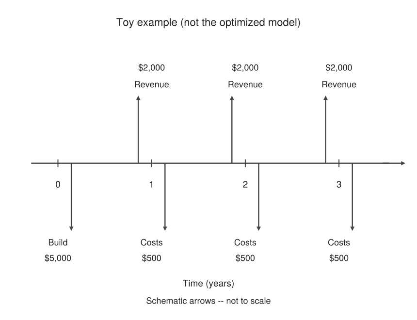
Annual operating surplus \(G(v)\) is accounted for at year ends \(j=1,\ldots,T\), with weight \(\nu^{j}\). Summing those weights over the horizon gives the annuity factor, the present value of one dollar received at each year end: \[ W_T=\sum_{j=1}^{T}\nu^{j} =\begin{cases} \dfrac{1-(1+\rho)^{-T}}{\rho},&\rho>0,\\ T,&\rho=0. \end{cases} \] The debt side also needs the finite geometric sum \[ \Sigma_n(z)=\sum_{k=0}^{n-1}z^k =\begin{cases} (1-z^n)/(1-z),&z\ne1,\\ n,&z=1. \end{cases} \] \(\Sigma_n(z)\) is an ordinary finite geometric sum; the ratio-one case \(z=1\) is separated only to avoid dividing by zero. Writing \(\Sigma_T\) in the debt coefficients just means this sum with \(n=T\), that is \(\Sigma_T(z)=\sum_{k=0}^{T-1}z^k\), the \(T\) annual maintenance terms.
Maintenance is paid every year, stopping after the first payment under cleanup, and cleanup is paid at year 1, after that first payment. Define the discounted debt coefficients as \[ \begin{aligned} \bar\kappa(T,\rho;\mathrm{never})&=r\cdot\nu\Sigma_T(\nu\cdot(1+r)),\\ \bar\kappa(T,\rho;\mathrm{clean})&=r\cdot\nu+(1+r)\cdot \nu. \end{aligned} \] Write \(\bar\kappa(T,\rho;\mathrm{never})\) for the never-clean policy and \(\bar\kappa(T,\rho;\mathrm{clean})\) for the year-1 cleanup policy; below, \(\bar\kappa(T,\rho;p)\) is the coefficient for a given policy.
The two coefficients differ only in how many maintenance bills are discounted. Under never cleaning, the year-\(k\) bill \(r\cdot D_{k-1}\) is discounted by \(\nu^k\); since \(\nu^k\cdot(1+r)^{k-1}=\nu\,[\nu\cdot(1+r)]^{k-1}\), summing over \(k\) gives the never-clean coefficient \(r\cdot\nu\sum_{k=1}^{T}[\nu\cdot(1+r)]^{k-1}=r\cdot\nu\cdot\Sigma_T(\nu\cdot(1+r))\). Under year-1 cleanup, only two payments occur, both at year 1: the first maintenance \(r\cdot D_0\) and the stock-removal bill \(D_1=(1+r)\cdot D_0\), which discount to \(r\cdot\nu\) and \((1+r)\cdot \nu\), so cleanup contributes \(r\cdot\nu+(1+r)\cdot \nu\) and nothing later. The geometric ratio \(\nu\cdot(1+r)\) compares how much a dollar is discounted in a year (\(\nu\)) with how much the debt grows over that year (\(1+r\)). When \(\nu\cdot(1+r)=1\), equivalently \(\rho=r\), the two exactly offset: every term in the sum equals \(1\), so \(\Sigma_T(1)=T\) grows linearly instead of converging, and the never-clean debt coefficient diverges as the horizon lengthens.
Net present value (NPV) is \[ \operatorname{NPV}(v;T,\rho;p) =W_T\cdot G(v)-B(v)-\bar\kappa(T,\rho;p)\cdot D_0(v). \] Discounting applies to both revenue and baseline incident losses, through \(W_T\cdot G\), and to the extra maintenance and cleanup through \(\bar\kappa(T,\rho;p)\). The build cost stays at time zero. The three terms are the operating stream discounted by \(W_T\), the build payment at time zero, and the debt outflows discounted by \(\bar\kappa(T,\rho;p)\). Here the annual complexity-carry rate \(r\) is not the annual time value of money \(\rho\): one describes real maintenance and complexity costs, the other when the cash flows arrive, and they are not two charges on the same interest.
Discounting can change how investments rank. Replacing \(T\) by \(W_T\) and \(\kappa(T;p)\) by \(\bar\kappa(T,\rho;p)\) gives \[ \begin{aligned} \operatorname{NPV}'(v;T,\rho;p)&=(1-\bar\kappa(T,\rho;p))\cdot \Lambda\gamma\cdot e^{-\gamma v} -2\alpha W_T\cdot(v-v_{\text{opt}})\cdot g(q(v)),\\ \operatorname{NPV}''(v;T,\rho;p)&=W_T\cdot G''(v)+(\bar\kappa(T,\rho;p)-1)\cdot \Lambda\gamma^2\cdot e^{-\gamma v}. \end{aligned} \] The same dominance condition as before decides concavity. Discounting changes the marginal conditions in just two places: the horizon weight \(T\) becomes \(W_T\) and the debt coefficient \(\kappa(T;p)\) becomes \(\bar\kappa(T,\rho;p)\), so the rest of the optimization is unchanged. In particular, at \(\rho=0\) we have \(\nu=1\), so \(\nu^k=1\), \(W_T=T\), and every \(\bar\kappa(T,\rho;p)=\kappa(T;p)\); the discounted expression collapses to the undiscounted lifecycle profit.
Write \(\bar\kappa_{\infty}(p)=\lim_{T\to\infty}\bar\kappa(T,\rho;p)\) for the infinite-horizon debt coefficients: \(\bar\kappa_{\infty}(\mathrm{clean})=r\cdot\nu+(1+r)\cdot \nu\), already constant in \(T\), and \(\bar\kappa_{\infty}(\mathrm{never})=r\cdot\nu/[1-\nu\cdot(1+r)]\), finite exactly when \(\nu\cdot(1+r)<1\).
The undiscounted lifetime limits do not carry over unchanged to \(\rho>0\). With discounting, distant years contribute little: \(W_T\to1/\rho\) as \(T\to\infty\), so the operating stream has a finite present value. The cleanup coefficient \(\bar\kappa(T,\rho;\mathrm{clean})\) is already constant in \(T\). The never-clean coefficient tends to the finite limit \(r\cdot\nu/[1-\nu\cdot(1+r)]\) only when \(\nu\cdot(1+r)<1\), that is, when the discount rate exceeds the debt rate (\(\rho>r\)). If instead \(\nu\cdot(1+r)\geq1\) (equivalently \(\rho\leq r\)), the discounted maintenance sum diverges, linearly in the number of payments at equality, so the debt cost grows without bound and the optimum is driven to \(v=0\). When \(\rho>r\), the limiting choice maximizes the finite objective \(G(v)/\rho-B(v)-\bar\kappa_{\infty}(p)\cdot D_0(v)\), which need not be the best-quality level or zero.
8.4 A Ten-Year Investment Example
I use the same illustrative quality, build, revenue, incident-rate, and per-incident cost parameters as before and run the product for \(T=10\) years. The debt rate is \(r=0.30\) per year: maintenance is paid once a year and compound complexity grows by 30% each year. For simplicity, I set \(\rho=0\), so neither revenue nor costs are discounted and cash dollars at every date get equal weight. These parameters are assumptions, not empirical estimates:
| Parameters | Assumed values |
|---|---|
| Quality | \(q_{\max}=\alpha=1\), \(v_{\text{opt}}=0.3\) |
| Upfront build | \(B_{\max}=\$100{,}000\), \(B_{\min}=\$20{,}000\), \(\gamma=2\) |
| Annual revenue | \(s=1\), \(\bar R_{\max}=\$100{,}000\)/year, \(\delta=2\) |
| Baseline incidents | \(\lambda_0=10\) incidents/year, \(\mu=\$5{,}000\)/incident, \(\beta=1\) |
| Debt stock and burden | \(D_0(v)=\Lambda\cdot(1-e^{-2v})\); \(r=0.30\) per year |
| Lifetime and discounting | \(T=10\) years, \(\rho=0\) (annual; no cash-flow discounting) |
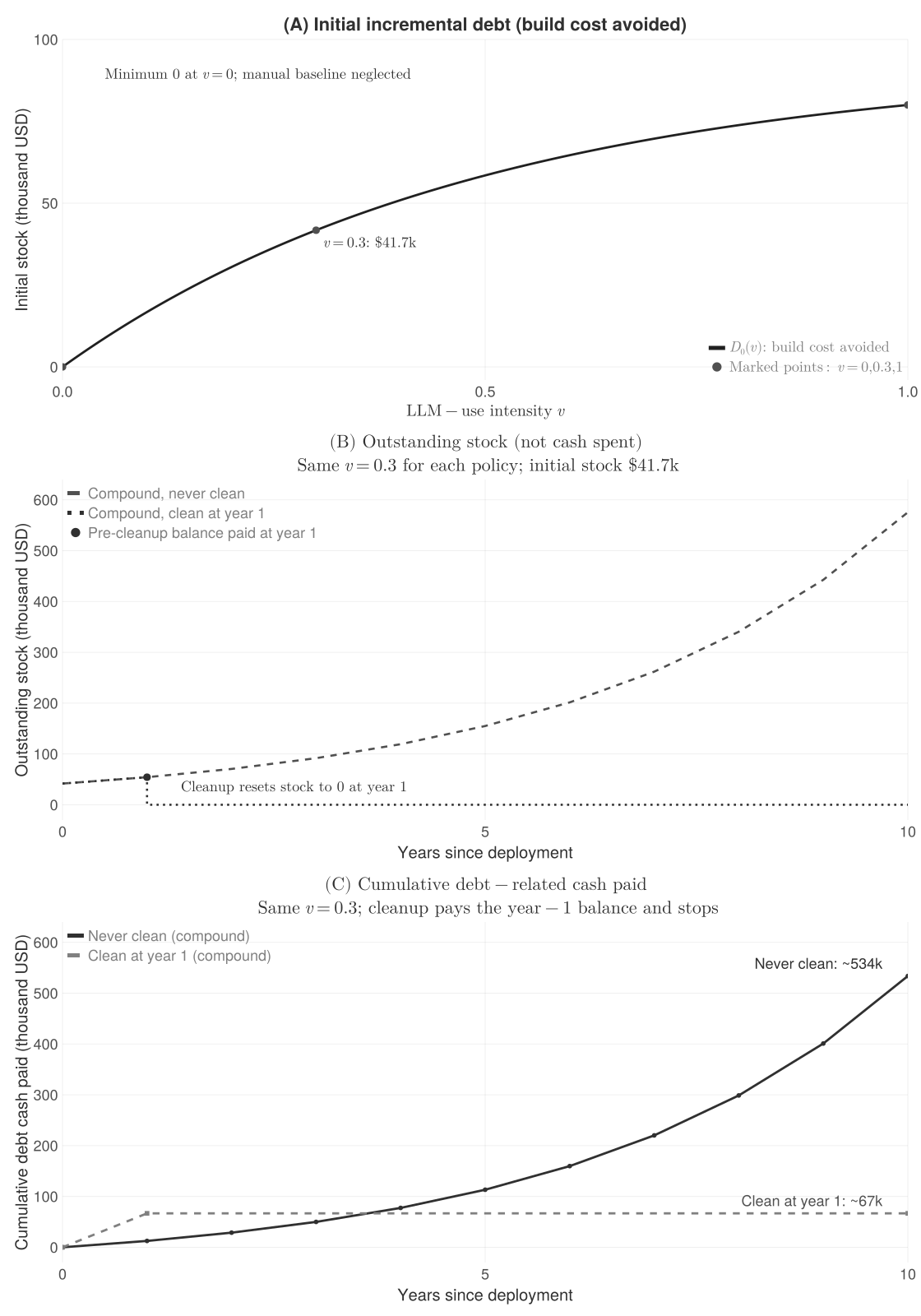
For a fixed \(v\), annual expected revenue \(\bar R(v)\) and ordinary incident expense \(\ell(v)\) stay the same across these ten years. They differ between investments because each policy gets its own optimal \(v\). Build spending happens at time zero, while operating receipts and baseline losses land at each year end. Maintenance happens at \(t=1,2,\ldots,10\) under never cleaning, or at \(t=1\) under cleanup. Cleanup occurs at the end of year 1, after the first maintenance payment, and modeled debt maintenance then stops. There is no retirement cleanup charge.
Here \(W_{10}=10\) and \(\bar\kappa(T,\rho;p)=\kappa(T;p)\). There are two debt coefficients, for compound never and compound cleanup: \(\kappa(T;\mathrm{never})\approx12.785849\) and \(\kappa(T;\mathrm{clean})=1.6\). I optimize each policy separately by solving its own marginal balance: \[ (1-\kappa(T;p))\cdot \Lambda\gamma\cdot e^{-2v} =20(v-0.3)\left[200{,}000e^{-2q(v)}+50{,}000e^{-q(v)}\right], \qquad q(v)=1-(v-0.3)^2. \] Because the debt cash is proportional to the build-cost saving, the debt term enters the marginal condition as \((1-\kappa(T;p))\cdot \Lambda\gamma\cdot e^{-\gamma v}\), not as a constant \(d\kappa(T;\mathrm{never})\). Compound-never has the largest coefficient, \(\kappa(T;\mathrm{never})\approx12.786\), and its corner marginal value is strongly negative, \(\Pi_{\mathrm{debt}}'(0;T,\mathrm{never})\approx-\$1{,}865{,}699\), so it corners at \(v^*=0\). Compound-cleanup has \(\kappa(T;\mathrm{clean})=1.6\) and \(\Pi_{\mathrm{debt}}'(0;T,\mathrm{clean})\approx\$204{,}162\), so it settles inside at \(v^*\approx0.222494\). The ten-year operating surplus is all ten annual expected revenues less all ten ordinary incident expenses. Debt cash spending is the extra maintenance plus any cleanup. All monetary entries are in USD, rounded to cents, and computed from the unrounded optima. Each policy row in the tables below is optimized over \(v\).
| Debt policy | Optimal \(v^*\) | Ten-year operating surplus | Upfront build | Total debt cash spending | Lifecycle profit |
|---|---|---|---|---|---|
| Compound, never clean | 0.00000000 | \(\$636{,}712.14\) | \(\$100{,}000.00\) | \(\$0.00\) | \(\$536{,}712.14\) |
| Compound, clean at year 1 | 0.22249421 | \(\$677{,}980.95\) | \(\$66{,}769.24\) | \(\$53{,}169.21\) | \(\$558{,}042.50\) |
Because \(D_0(0)=0\), the compound-never corner at \(v^*=0\) is also the manual, LLM-free choice: at these horizons, never cleaning makes LLM use unprofitable and the policy collapses to ordinary manual coding.
Re-optimizing the same two policies at a longer horizon shows what happens when debt is not paid down. At \(T=20\) years, compound-never again takes the corner \(v^*=0\) and gives the lower lifecycle profit, while cleanup recovers value:
| Debt policy | Optimal \(v^*\) | Total debt cash spending | Lifecycle profit |
|---|---|---|---|
| Compound, never clean | 0.00000000 | \(\$0.00\) | \(\$1{,}173{,}424.27\) |
| Compound, clean at year 1 | 0.26406963 | \(\$60{,}738.27\) | \(\$1{,}237{,}498.13\) |
8.4.1 The Two Compound Investments as Cash Streams
Revenue is an expected cash inflow, while build spending, ordinary incident expense, maintenance, and cleanup are expected cash outflows. The optimized choices differ by policy, and here compound-never corners at \(v^*=0\), so I illustrate the compound debt mechanics at a common fixed use level \(v=0.3\) over \(T=10\) years rather than at independently optimized choices. The two schedules below are fixed-use, not optimized; the policy tables above stay optimized. Amounts are positive magnitudes, and subtracting the outflows gives net cash. Time zero contains only the upfront build payment. Maintenance formulas use the unrounded \(D_0\), and the displayed monetary checks are rounded to cents.
Compound debt, never clean (fixed \(v=0.3\), \(D_0=\$41{,}744.58\)):
| Timing (years after deployment) | Cash flow | Amount (USD) |
|---|---|---|
| \(t=0\) | Build outflow | \(\$58{,}255.42\) |
| Each year end 1–10 | Revenue inflow | \(\$86{,}466.47\) per year |
| Each year end 1–10 | Ordinary incident outflow | \(\$18{,}393.97\) per year |
| \(t=k\), \(k=1,\ldots,10\) | Maintenance outflow | \(r\cdot(1+r)^{k-1}\cdot D_0\) |
| \(t=1\) | First maintenance check | \(\$12{,}523.38\) |
| \(t=10\) | Final maintenance check | \(\$132{,}804.13\) |
| None | Cleanup outflow | \(\$0\) |
Annual operating surplus is \(G\approx\$68{,}072.50\). Year ends have net cash \(G-M_k\): the checks are \(\$55{,}549.12\) at \(t=1\) and \(-\$64{,}731.63\) at \(t=10\). Total debt cash spending is \(\$533{,}739.96\), which exceeds the fixed-use lifecycle profit of \(\$88{,}729.62\), showing how fast a 30% compounding burden grows. The maintenance checks illustrate the formula rather than adding payments.
Compound debt, clean at year 1 (fixed \(v=0.3\), \(D_0=\$41{,}744.58\)):
| Timing (years after deployment) | Cash flow | Amount (USD) |
|---|---|---|
| \(t=0\) | Build outflow | \(\$58{,}255.42\) |
| Each year end 1–10 | Revenue inflow | \(\$86{,}466.47\) per year |
| Each year end 1–10 | Ordinary incident outflow | \(\$18{,}393.97\) per year |
| \(t=1\) | Maintenance outflow | \(r\cdot D_0=\$12{,}523.38\) |
| \(t=1\), after maintenance | Cleanup outflow | \((1+r)\cdot D_0=\$54{,}267.96\) |
| \(t>1\) | Maintenance and cleanup outflows | \(\$0\) |
Annual operating surplus is \(G\approx\$68{,}072.50\). Net cash is \(G-M_1-D_1\) at \(t=1\) and \(G\) at year ends 2–10: the checks are \(\$1{,}281.16\) and \(\$68{,}072.50\). Again, the check rows do not add payments. The single maintenance bill is \(\$12{,}523.38\), and the cleanup bill comes on top of it, giving \(\$66{,}791.33\) in debt cash spending.
The stock \(D_0\) is not an extra cash charge. At this fixed \(v=0.3\), the compound-cleanup debt cash of \(\$66{,}791.33\) is about 12% of its lifecycle profit of \(\$555{,}678.25\), while compound-never debt cash of \(\$533{,}739.96\) exceeds its lifecycle profit of \(\$88{,}729.62\). Summing the unrounded fixed-use cash streams gives lifecycle profits, also NPVs at \(\rho=0\), of \(\$88{,}729.62\) for never and \(\$555{,}678.25\) for cleanup; independent rounding can make the displayed checks differ slightly from the totals.
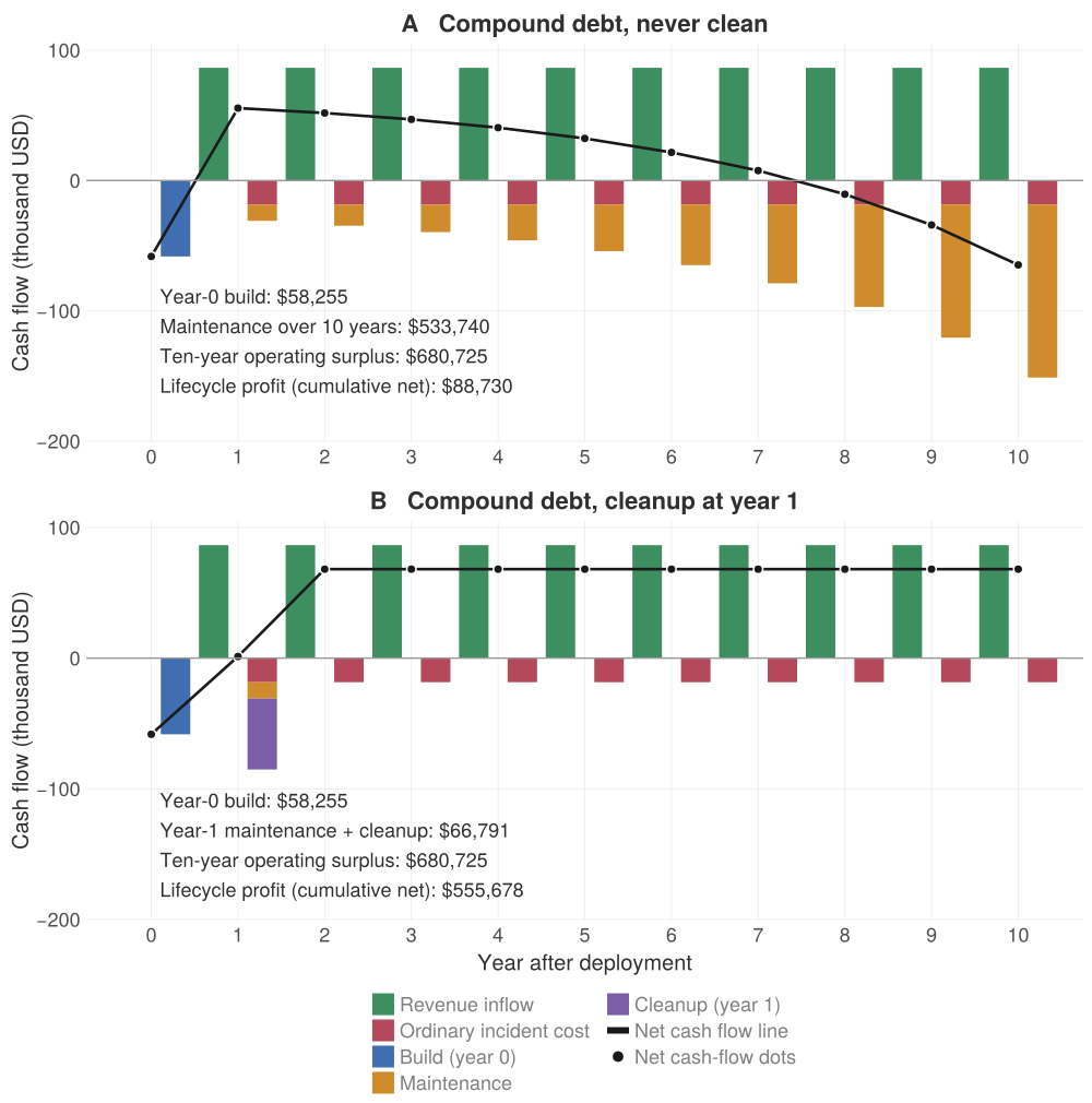
Between the optimized policies at \(T=10\), compound cleanup improves lifecycle profit by about \(\$21{,}330.36\). Compound-never is already at the corner \(v^*=0\), so never cleaning means abandoning LLM use.
Cleanup is not always best over a short lifetime. The analytical compound threshold derived above is \(T>1+\log 2/\log(1+r)\approx3.641927\) years without discounting: the first annual-grid horizon at which year-1 cleanup is cheaper than never cleaning, at any fixed \(v\) with \(D_0(v)>0\), is 4 years. This debt-only comparison applies on annual horizons independently of the operating schedule.
In plain terms, code that will not be used for long is cheaper to leave uncleaned, because the early cleanup bill is not repaid by enough avoided maintenance; only code that lives long enough for the compounding burden to accumulate makes early cleanup worth its cost.
8.4.2 What the Zero-Discount Assumption Leaves Out
Money committed to building or cleaning software cannot earn interest in a bank or fund another investment at the same time. A better available return raises the opportunity cost of spending now rather than receiving money later, and can make an upfront investment less attractive. Cash-flow discounting handles this timing by applying \((1+\rho)^{-t}\), with effective annual \(\rho\) and \(t\) in years, to every inflow and outflow at its actual date, not only to revenue. It does not automatically favor never cleaning: earlier cleanup spending can prevent larger later outflows. The debt rate \(r\) describes real maintenance and complexity growth, while \(\rho\) describes the required financial return; they are different parameters.
Revenue uncertainty belongs in \(s\) or in the expected cash-flow forecasts. A risk premium can also be part of the required return \(\rho\) if that is justified, but uncertainty and discounting are not interchangeable and should not be counted twice. The zero-discount comparison above isolates the debt trade-off for simplicity. Whether its ranking survives a positive discount rate needs a separate sensitivity analysis of all cash flows and, when optimizing the investment, a fresh optimum for each policy; I do not assume the ranking is invariant.
9 Conclusion
For me, the main lesson is that there is no universally optimal amount of LLM use. Getting software built faster is only part of the decision. Development savings, expected revenue, and the consequences of incidents need to be considered together.
Much of this may seem fairly obvious. The value of writing it down mathematically is that it forces the argument’s assumptions into the open, where they can be checked.
Low-impact experiments with inexpensive fixes and uncertain commercial payoff can support greater reliance on LLMs, if the assumed savings and quality effects hold. When failures have serious consequences, or better quality brings greater expected revenue, preserving quality and investing in oversight become more important. The best-quality approach may still use LLMs; it need not be entirely manual. Under the assumption that quality is highest without LLM use, increasingly costly incidents instead push the unconstrained choice toward no use.
An upfront budget changes what is feasible. When it excludes the preferred approach, it can force a higher-use, lower-quality choice without making that choice the safest or the most profitable without the constraint. A favorable average financial outcome is not enough to justify accepting a risk of unacceptable catastrophic harm. Regulatory and safety requirements may rule out choices that this economic model would otherwise allow.
I also worry about the incentives around these choices. With LLM assistance, a working prototype can make shortcuts look like productivity gains worth rewarding, while maintenance costs remain deferred. That can become a slippery slope: each apparent success normalizes more shortcuts. Engineers who later inherit fragile code may spend largely invisible effort reviewing, fixing, and refactoring it to repay technical debt. This can be especially frustrating for competent, conscientious engineers if delivery speed still counts for more than maintainability. The tool alone does not cause this problem, and a deliberately scoped, time-limited prototype can be a rational choice. That is different from passing unplanned debt to others. Rather than shaming LLM users, I would make cleanup time, resources, and accountability visible in the original decision.
The curves and parameters here are illustrative, not empirical estimates. I see this framework as a way to clarify which assumptions drive a decision, not as a verdict on LLMs. In practice, I would estimate the trade-offs using evidence from the actual development context, including the effort spent reviewing, testing, and repairing code. Those estimates, and the level of assistance and oversight, should be revisited as the software and its deployment environment change.
I should be clear that this analysis leans on many simplifying assumptions. Incidents follow a homogeneous Poisson process in a fixed environment with a constant expected cost per incident; quality is a single scalar; the quality-response and build-cost curves are monotone in the ways I assumed; debt compounds at a single rate; and the base case sets discounting aside. These choices kept the model tractable and let me reach analytic results, but they are not the whole story. I would find it interesting to build more flexible versions with time-varying rates, heterogeneous costs, changing quality, richer treatment of risk and tails, and calibration to real data, then ask whether the conclusions above survive or shift.
One way to use these results is to give each parameter a prior distribution for a specific application, or even for a component of an application, using the best guesses of people who know the domain. A prior predictive simulation can then draw many parameter combinations, compute the optimal LLM use in each scenario, and summarize the draws as a credible interval for the optimal level. Because the LLM-use and quality variables are abstract and the model rests on strong structural assumptions, that interval is best read as a general guide to how much LLM use a team might accept, not a precise instruction. It also does not say concretely how to use LLMs while coding, which makes the recommendation hard to enforce or interpret. That is not a reason to abandon the economic reasoning though; it means more research is needed to make it more useful, perhaps by tailoring it to specific patterns of LLM use and specific applications.
I would extend this reasoning to content creation and AI-assisted research paper writing. Returns can include reach, recognition, and credibility, or lost trust and reputational harm when readers dislike AI-generated content, depending on their attitudes. Time saved must be balanced against checking accuracy, originality, authorship, and transparency; research integrity obligations are not an optional economic bargain. The equations, quality and cost functions, and parameters would need tailoring to each domain. Working with multiple quality criteria \(q\), multi-dimensional LLM use variable \(v\), different domains of AI use, and more flexible mathematical models with less assumptions are all promising research directions to extend this work.
References
Becker, J., Rush, N., Barnes, E., & Rein, D. (2025). Measuring the impact of early-2025 AI on experienced open-source developer productivity. arXiv:2507.09089. https://arxiv.org/abs/2507.09089
Boehm, B. W. (1981). Software Engineering Economics. Englewood Cliffs, NJ, USA: Prentice-Hall. ISBN 978-0-13-822122-5.
Boyd, S., & Vandenberghe, L. (2004). Convex Optimization. Cambridge, U.K.: Cambridge University Press. ISBN 978-0-521-83378-3.
Breiman, L. (2001). Statistical modeling: The two cultures (with comments and a rejoinder by the author). Statistical Science, 16(3), 199–231. https://doi.org/10.1214/ss/1009213726
Chen, R. T. Q., Rubanova, Y., Bettencourt, J., & Duvenaud, D. (2018). Neural ordinary differential equations. In Advances in Neural Information Processing Systems 31 (NeurIPS 2018), Montreal, QC, Canada, 6572–6583. arXiv:1806.07366. https://proceedings.neurips.cc/paper_files/paper/2018/hash/69386f6bb1dfed68692a24c8686939b9-Abstract.html
Cunningham, W. (1992). The WyCash portfolio management system. In Addendum to the Proc. ACM Conf. Object-Oriented Programming Systems, Languages, and Applications (OOPSLA ’92), Vancouver, BC, Canada, 29–30. https://doi.org/10.1145/157709.157715
Dijkstra, E. W. (1972). The humble programmer. Commun. ACM, 15(10), 859–866. https://doi.org/10.1145/355604.361591
Fowler, M. (2009). Technical debt quadrant. martinfowler.com. https://martinfowler.com/bliki/TechnicalDebtQuadrant.html
GitClear (2025). AI Copilot code quality: 2025 data suggests 4x growth in code clones. GitClear. https://www.gitclear.com/ai_assistant_code_quality_2025_research
Goodenough, J. B., & Gerhart, S. L. (1975). Toward a theory of test data selection. IEEE Trans. Softw. Eng., SE-1(2), 156–173. https://doi.org/10.1109/TSE.1975.6312836
Kapoor, A., & Narayanan, A. (2023). Leakage and the reproducibility crisis in machine-learning-based science. Patterns, 4(9), art. no. 100804. https://doi.org/10.1016/j.patter.2023.100804
Koh, P. W., et al. (2021). WILDS: A benchmark of in-the-wild distribution shifts. In Proc. 38th Int. Conf. Machine Learning (ICML 2021), PMLR 139, 5637–5664. arXiv:2012.07421. https://proceedings.mlr.press/v139/koh21a.html
Kruchten, P., Nord, R. L., & Ozkaya, I. (2012). Technical debt: From metaphor to theory and practice. IEEE Software, 29(6), 18–21. https://doi.org/10.1109/MS.2012.167
Kuhn, H. W., & Tucker, A. W. (1951). Nonlinear programming. In Proceedings of the Second Berkeley Symposium on Mathematical Statistics and Probability, J. Neyman, Ed. Berkeley, CA, USA: University of California Press, 481–492. https://doi.org/10.1525/9780520411586-036
Mehta, I. (2025). A quarter of startups in YC’s current cohort have codebases that are almost entirely AI-generated. TechCrunch. https://techcrunch.com/2025/03/06/a-quarter-of-startups-in-ycs-current-cohort-have-codebases-that-are-almost-entirely-ai-generated/
Mould, D. R., & Upton, R. N. (2012). Basic concepts in population modeling, simulation, and model-based drug development. CPT: Pharmacometrics & Systems Pharmacology, 1(9), art. no. e6. https://doi.org/10.1038/psp.2012.4
Myers, G. J., Sandler, C., & Badgett, T. (2011). The Art of Software Testing, 3rd ed. Hoboken, NJ, USA: John Wiley & Sons. ISBN 978-1-118-03196-4.
Paradis, E., et al. (2024). How much does AI impact development speed? An enterprise-based randomized controlled trial. arXiv:2410.12944. https://arxiv.org/abs/2410.12944
Pearce, H., Ahmad, B., Tan, B., Dolan-Gavitt, B., & Karri, R. (2022). Asleep at the keyboard? Assessing the security of GitHub Copilot’s code contributions. In Proc. 2022 IEEE Symp. Security and Privacy (SP), 754–768. https://doi.org/10.1109/SP46214.2022.9833571
Peng, S., Kalliamvakou, E., Cihon, P., & Demirer, M. (2023). The impact of AI on developer productivity: Evidence from GitHub Copilot. arXiv:2302.06590. https://arxiv.org/abs/2302.06590
Perry, N., Srivastava, M., Kumar, D., & Boneh, D. (2023). Do users write more insecure code with AI assistants? In Proc. 2023 ACM SIGSAC Conf. Computer and Communications Security (CCS ’23), 2785–2799. https://doi.org/10.1145/3576915.3623157
Quiñonero-Candela, J., Sugiyama, M., Schwaighofer, A., & Lawrence, N. D., Eds. (2009). Dataset Shift in Machine Learning. Cambridge, MA, USA: MIT Press. ISBN 978-0-262-17005-5.
Rackauckas, C., et al. (2020). Universal differential equations for scientific machine learning. arXiv:2001.04385 (v4, Nov. 2021). https://arxiv.org/abs/2001.04385
Raissi, M., Perdikaris, P., & Karniadakis, G. E. (2019). Physics-informed neural networks: A deep learning framework for solving forward and inverse problems involving nonlinear partial differential equations. Journal of Computational Physics, 378, 686–707. https://doi.org/10.1016/j.jcp.2018.10.045
Sculley, D., et al. (2015). Hidden technical debt in machine learning systems. In Advances in Neural Information Processing Systems 28 (NIPS 2015), Montreal, QC, Canada, 2503–2511. https://papers.nips.cc/paper_files/paper/2015/hash/86df7dcfd896fcaf2674f757a2463eba-Abstract.html
Sheiner, L. B., & Steimer, J.-L. (2000). Pharmacokinetic/pharmacodynamic modeling in drug development. Annual Review of Pharmacology and Toxicology, 40, 67–95. https://doi.org/10.1146/annurev.pharmtox.40.1.67
Vaithilingam, P., Zhang, T., & Glassman, E. L. (2022). Expectation vs. experience: Evaluating the usability of code generation tools powered by large language models. In CHI EA ’22: Extended Abstracts of the 2022 CHI Conf. Human Factors in Computing Systems, 1–7. https://doi.org/10.1145/3491101.3519665
Ziegler, A., et al. (2024). Measuring GitHub Copilot’s impact on productivity. Commun. ACM, 67(3), 54–63. https://doi.org/10.1145/3633453